Bayesian inference with interacting particle systems
Source:R/rbiips-package.r
rbiips is an interface with the Biips C++ libraries for analysing Bayesian graphical models using advanced particle methods.
Details
Biips is a general software for Bayesian inference with interacting particle systems, a.k.a. sequential Monte Carlo (SMC) methods. It aims at popularizing the use of these methods to non-statistician researchers and students, thanks to its automated “black box” inference engine. It borrows from the BUGS/JAGS software, widely used in Bayesian statistics, the statistical modeling with graphical models and the language associated with their descriptions.
See the Biips website for more information.
The typical workflow is the following:
Define the model in BUGS language (see the JAGS User Manual for help) and the data.
Add custom functions or distributions with
biips_add_functionandbiips_add_distribution.Compile the model with
biips_modelRun inference algorithms:
Analyse sensitivity to parameters with
biips_smc_sensitivity.Run SMC filtering and smoothing algorithms with
biips_smc_samples.Run particle MCMC algorithms with
biips_pimh_samplesorbiips_pmmh_samples.
Diagnose and analyze the output obtained as
smcarrayandmcmcarrayobjects withbiips_diagnosis,biips_summary,biips_density,biips_histandbiips_table
References
Adrien Todeschini, François Caron, Marc Fuentes, Pierrick Legrand, Pierre Del Moral (2014). Biips: Software for Bayesian Inference with Interacting Particle Systems. arXiv preprint arXiv:1412.3779. URL http://arxiv.org/abs/1412.3779
See also
biips_add_function, biips_add_distribution,
biips_model, biips_smc_sensitivity, biips_smc_samples,
biips_pimh_samples, biips_pmmh_samples, smcarray,
mcmcarray, biips_diagnosis, biips_summary,
biips_density, biips_hist, biips_table,
Biips website,
JAGS User Manual
Examples
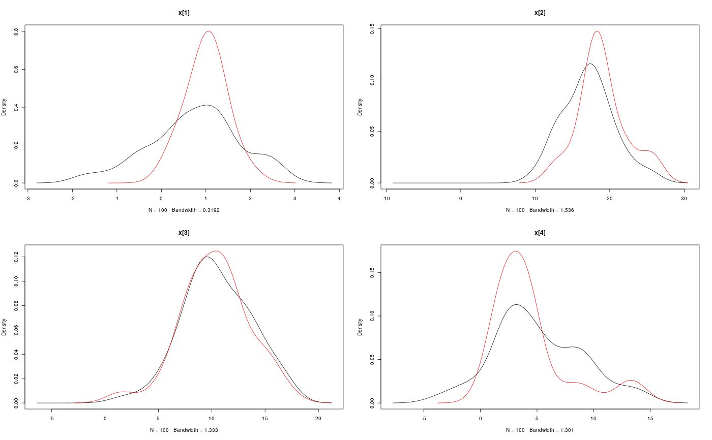
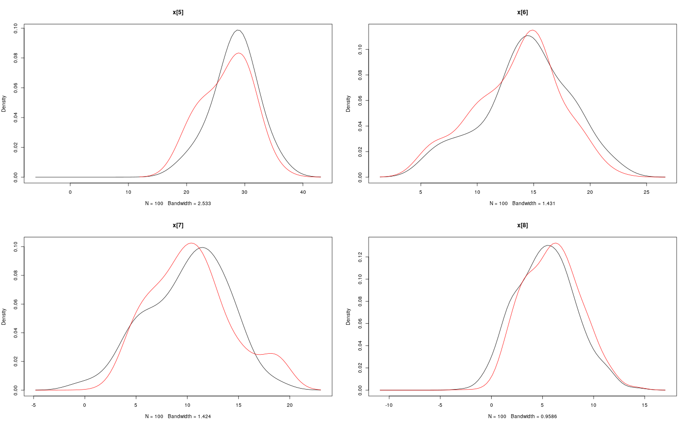
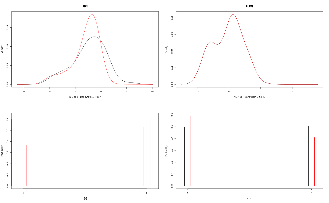
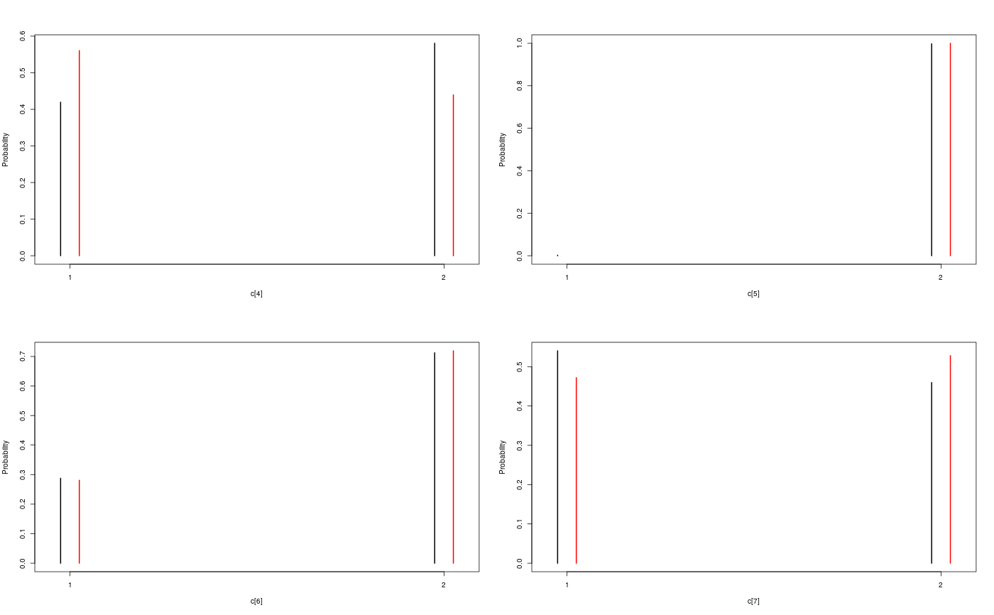
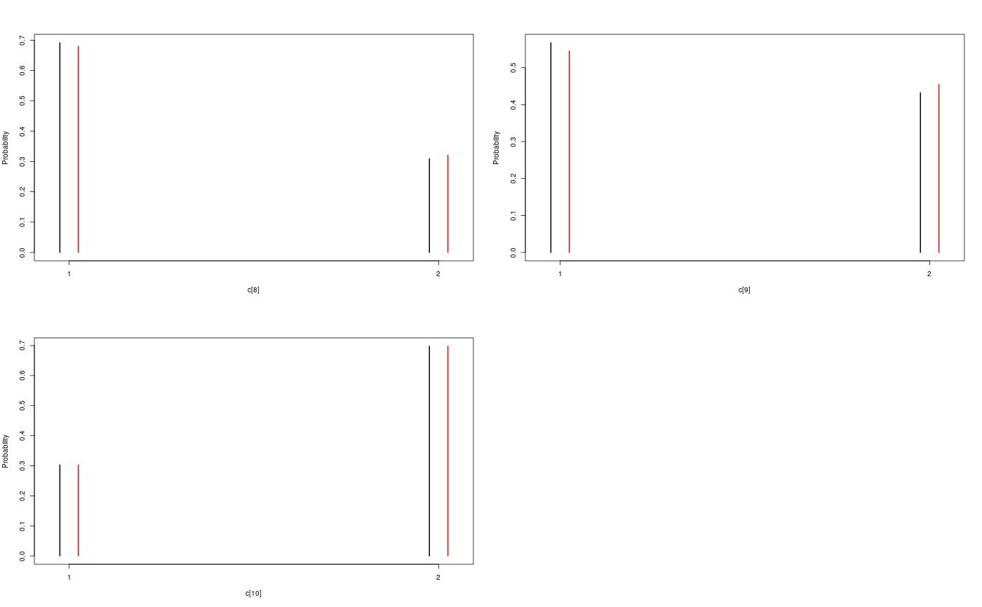
#' # Add custom functions and distributions to BUGS language #' Add custom function `f` f_dim <- function(x_dim, t_dim) { # Check dimensions of the input and return dimension of the output of function f stopifnot(prod(x_dim) == 1, prod(t_dim) == 1) x_dim } f_eval <- function(x, t) { # Evaluate function f 0.5 * x + 25 * x/(1 + x^2) + 8 * cos(1.2 * t) } biips_add_function('f', 2, f_dim, f_eval)#> * Added function f#' Add custom sampling distribution `dMN` dMN_dim <- function(mu_dim, Sig_dim) { # Check dimensions of the input and return dimension of the output of # distribution dMN stopifnot(prod(mu_dim) == mu_dim[1], length(Sig_dim) == 2, mu_dim[1] == Sig_dim) mu_dim } dMN_sample <- function(mu, Sig) { # Draw a sample of distribution dMN mu + t(chol(Sig)) %*% rnorm(length(mu)) } biips_add_distribution('dMN', 2, dMN_dim, dMN_sample)#> * Added distribution dMN#' # Compile model modelfile <- system.file('extdata', 'hmm_f.bug', package = 'rbiips') stopifnot(nchar(modelfile) > 0) cat(readLines(modelfile), sep = '\n')#> var c_true[tmax], x_true[tmax], c[tmax], x[tmax], y[tmax] #> #> data #> { #> x_true[1] ~ dnorm(0, 1/5) #> y[1] ~ dnorm(x_true[1], exp(logtau_true)) #> for (t in 2:tmax) #> { #> c_true[t] ~ dcat(p) #> x_true[t] ~ dnorm(f(x_true[t-1], t-1), ifelse(c_true[t]==1, 1/10, 1/100)) #> y[t] ~ dnorm(x_true[t]/4, exp(logtau_true)) #> } #> } #> #> model #> { #> logtau ~ dunif(-3, 3) #> x[1] ~ dnorm(0, 1/5) #> y[1] ~ dnorm(x[1], exp(logtau)) #> for (t in 2:tmax) #> { #> c[t] ~ dcat(p) #> x[t] ~ dnorm(f(x[t-1], t-1), ifelse(c[t]==1, 1/10, 1/100)) #> y[t] ~ dnorm(x[t]/4, exp(logtau)) #> } #> }data <- list(tmax = 10, p = c(.5, .5), logtau_true = log(1), logtau = log(1)) model <- biips_model(modelfile, data, sample_data = TRUE)#> * Parsing model in: /home/adrien/Dropbox/workspace/rbiips/inst/extdata/hmm_f.bug #> * Compiling data graph #> Declaring variables #> Resolving undeclared variables #> Allocating nodes #> Graph size: 94 #> Sampling data #> Reading data back into data table #> * Compiling model graph #> Declaring variables #> Resolving undeclared variables #> Allocating nodes #> Graph size: 105#' # SMC algorithm n_part <- 100 out_smc <- biips_smc_samples(model, c('x', 'c[2:10]'), n_part, type = 'fs', rs_thres = 0.5, rs_type = 'stratified')#> * Assigning node samplers #> * Running SMC forward sampler with 100 particles #> |--------------------------------------------------| 100% #> |**************************************************| 10 iterations in 0.03 sbiips_diagnosis(out_smc)#> * Diagnosis of variable: c[2:10] #> Filtering: POOR #> The minimum effective sample size is too low: 19.0924 #> Estimates may be poor for some variables. #> You should increase the number of particles #> . Smoothing: POOR #> The minimum effective sample size is too low: 15.6918 #> Estimates may be poor for some variables. #> You should increase the number of particles #> .* Diagnosis of variable: x[1:10] #> Filtering: POOR #> The minimum effective sample size is too low: 19.0924 #> Estimates may be poor for some variables. #> You should increase the number of particles #> . Smoothing: POOR #> The minimum effective sample size is too low: 15.6918 #> Estimates may be poor for some variables. #> You should increase the number of particles #> .biips_summary(out_smc)#> c[2:10] filtering smcarray: #> $mode #> [1] 2 2 2 2 2 1 1 1 2 #> #> Marginalizing over: particle(100) #> #> c[2:10] smoothing smcarray: #> $mode #> [1] 2 1 1 2 2 2 1 1 2 #> #> Marginalizing over: particle(100) #> #> #> x filtering smcarray: #> $mean #> [1] 0.7551302 17.1366606 10.5198695 5.0518616 28.2675467 14.2984628 #> [7] 10.0172888 5.3017900 -2.3033567 -20.3389452 #> #> Marginalizing over: particle(100) #> #> x smoothing smcarray: #> $mean #> [1] 1.012813 18.994901 10.283799 4.409567 26.870470 13.501392 #> [7] 10.385271 5.940201 -2.996455 -20.338945 #> #> Marginalizing over: particle(100) #> #>