Objects for representing SMC output.

Source: R/smcarray-object.r

A smcarray object is used by the biips_smc_samples function to represent SMC output or particles of a given variable.

A smcarray.fsb object is a named list of smcarray objects with different types of monitoring for the same variable. Members in this list have names f (filtering), s (smoothing) or b (backward smoothing).

A smcarray.fsb.list object is a named list of smcarray.fsb objects for different monitored variables. It might also contain a member named log_marg_like with an estimate of the log marginal likelihood.

The methods apply identically to smcarray, smcarray.fsb or smcarray.fsb.list objects and return a named list with the same named members as the input object.

is.smcarray(object)

is.smcarray.fsb(object)

is.smcarray.fsb.list(object)

biips_diagnosis(object, ...)

# S3 method for smcarray
biips_diagnosis(object, ess_thres = 30, quiet = FALSE,
  ...)

# S3 method for smcarray.fsb
biips_diagnosis(object, type = "fsb", quiet = FALSE,
  ...)

# S3 method for smcarray.fsb.list
biips_diagnosis(object, type = "fsb",
  quiet = FALSE, ...)

biips_summary(object, ...)

# S3 method for smcarray
biips_summary(object, probs = c(), order = ifelse(mode,
  0, 1), mode = all(object$discrete), ...)

# S3 method for smcarray.fsb
biips_summary(object, ...)

# S3 method for smcarray.fsb.list
biips_summary(object, ...)

biips_table(x, ...)

# S3 method for smcarray
biips_table(x, ...)

biips_density(x, ...)

# S3 method for smcarray
biips_density(x, bw = "nrd0", ...)

# S3 method for smcarray.fsb
biips_table(x, ...)

# S3 method for smcarray.fsb
biips_density(x, bw = "nrd0", adjust = 1, ...)

# S3 method for smcarray.fsb.list
biips_table(x, ...)

# S3 method for smcarray.fsb.list
biips_density(x, bw = "nrd0", ...)

# S3 method for smcarray
summary(object, ...)

# S3 method for smcarray.fsb
summary(object, ...)

# S3 method for smcarray.fsb.list
summary(object, ...)

# S3 method for smcarray
density(x, ...)

# S3 method for smcarray.fsb
density(x, ...)

# S3 method for smcarray.fsb.list
density(x, ...)

Arguments

object, x	a smcarray, smcarray.fsb or smcarray.fsb.list object.
...	additional arguments to be passed to the default methods. See density, table
ess_thres	integer. Threshold on the Effective Sample Size (ESS). If all the ESS components are over ess_thres, the diagnostic is 'GOOD', otherwise it is 'BAD'. (default=30).
quiet	logical. Disable message display. (default=FALSE).
type	string containing the characters 'f' (fitering), 's' (smoothing) and/or 'b' (backward smoothing). Select the corresponding members of the input to be analysed. (default = 'fsb').
probs	vector of reals. probability levels in ]0,1[ for quantiles. (default = c())
order	integer. Moment statistics of order below or equal to order are returned. (default = 0 if all the components are discrete variables and 1 otherwise)
mode	logical. Activate computation of the mode, i.e. the most frequent value among the particles. (default = TRUE if all the components are discrete variables and FALSE otherwise)
bw	either a real with the smoothing bandwidth to be used or a string giving a rule to choose the bandwidth. See bw.nrd. (default='nrd0')
adjust	scale factor for the bandwidth. the bandwidth used is actually adjust*bw. This makes it easy to specify values like ‘half the default’ bandwidth. (default = 1)

Value

The methods apply identically to smcarray, smcarray.fsb or smcarray.fsb.list objects and return a named list with the same named members as the input object.

The function is.smcarray returns TRUE if the object is of class smcarray.

The function is.smcarray.fsb returns TRUE if the object is of class smcarray.fsb.

The function is.smcarray.fsb.list returns TRUE if the object is of class smcarray.fsb.list.

The method biips_diagnosis prints diagnosis of the SMC output and returns the minimum ESS value.

The method biips_summary returns univariate marginal statistics. The output innermost members are objects of class summary.smcarray. Assuming dim is the dimension of the variable, the summary.smcarray object is a list with the following members:

mean

array of size dim. The mean if order>=1.

var

array of size dim. The variance, if order>=2.

skew

array of size dim. The skewness, if order>=3.

kurt

array of size dim. The kurtosis, if order>=4.

probs

vector of quantile probabilities.

quant

list of arrays of size dim for each probability level in probs. The quantile values, if probs is not empty.

mode

array of size dim. The most frequent values for discrete components.

The method biips_table returns univariate marginal frequency tables or probability mass estimates of discrete variables. The output innermost members are objects of class table.smcarray. The method biips_density returns univariate marginal kernel density estimates. The output innermost members are objects of class density.smcarray. The method summary is an alias for biips_summary. The method density is an alias for biips_density.

Details

Assuming dim is the dimension of the monitored variable, a smcarray object is a list with the members:

values

array of dimension c(dim, n_part) with the values of the particles.

weights

array of dimension c(dim, n_part) with the weights of the particles.

ess

array of dimension dim with Effective Sample Sizes of the particles set.

discrete

array of dimension dim with logicals indicating discreteness of each component.

iterations

array of dimension dim with sampling iterations of each component.

conditionals

lists of the contitioning variables (observations). Its value is:

• for filtering: a list of dimension dim. each member is a character vector with the respective conditioning variables of the node array component.

• for smoothing/backward_smoothing: a character vector, the same for all the components of the node array.

name

string with the name of the variable.

lower

vector with the lower bounds of the variable.

upper

vector with the upper bounds of the variable.

type

string with the type of monitor ('filtering', 'smoothing' or 'backward_smoothing').

For instance, if out_smc is a smcarray.fsb.list object, one can access the values of the smoothing particles for the variable 'x' with: out_smc$x$s$values.

See also

density

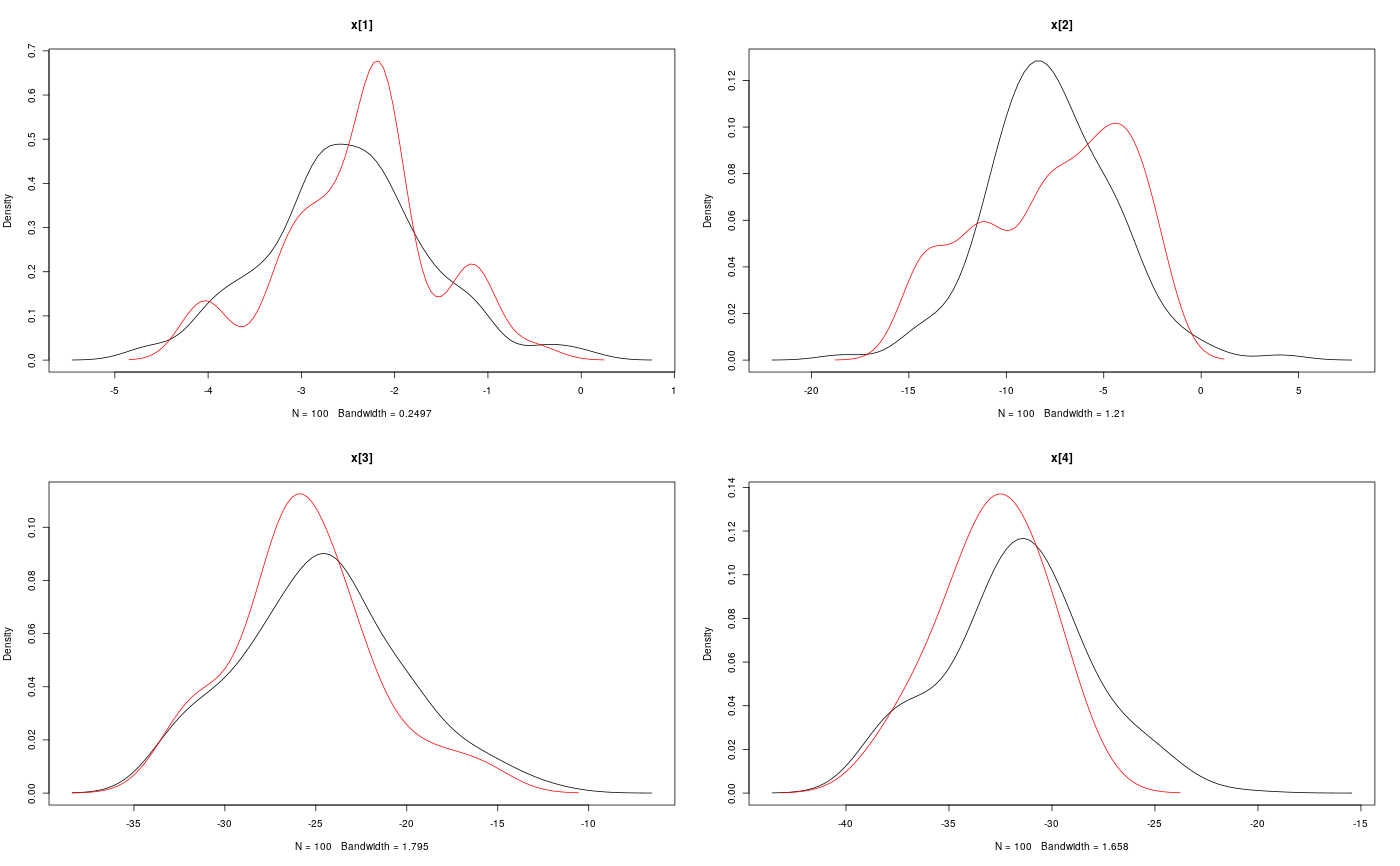
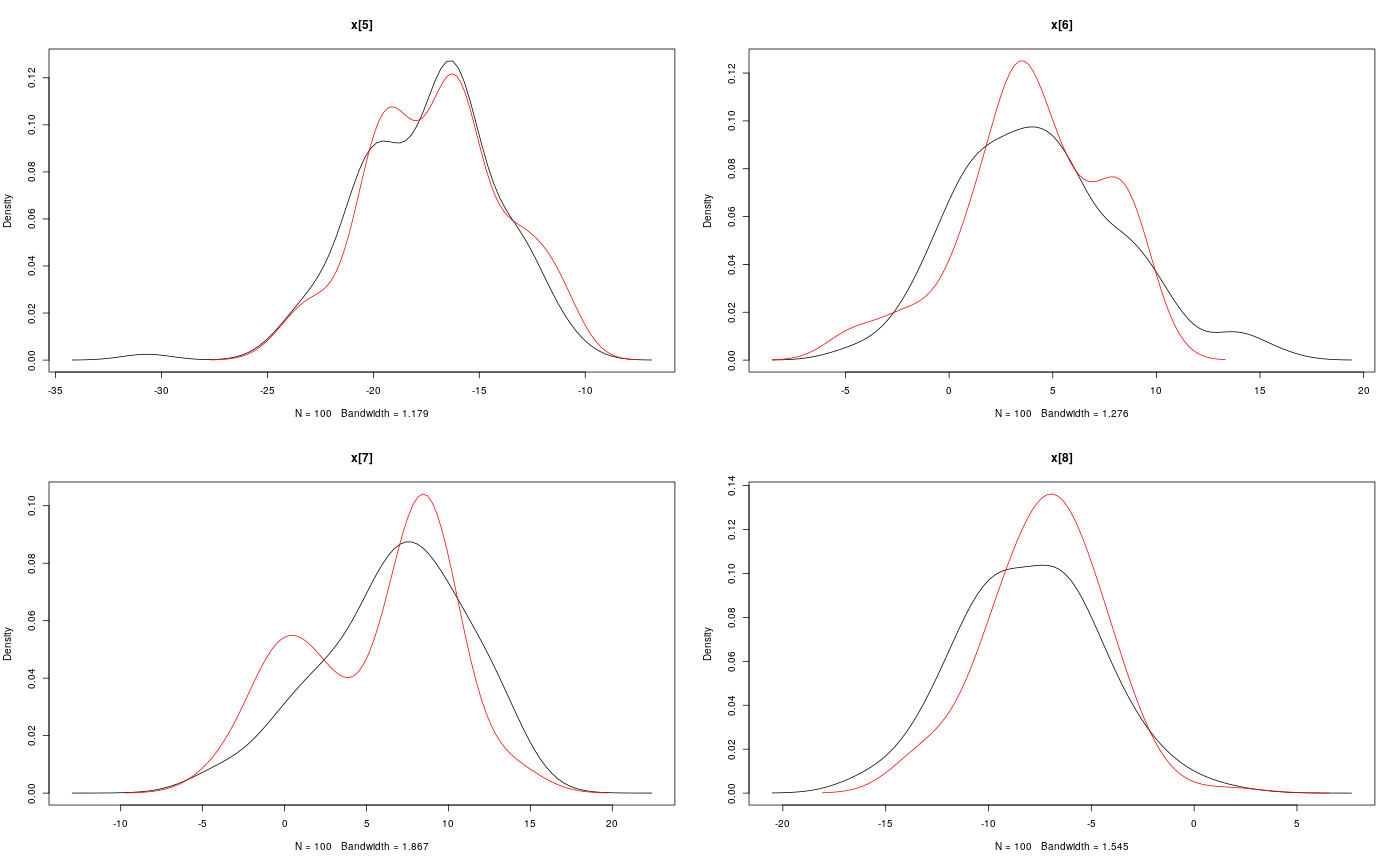
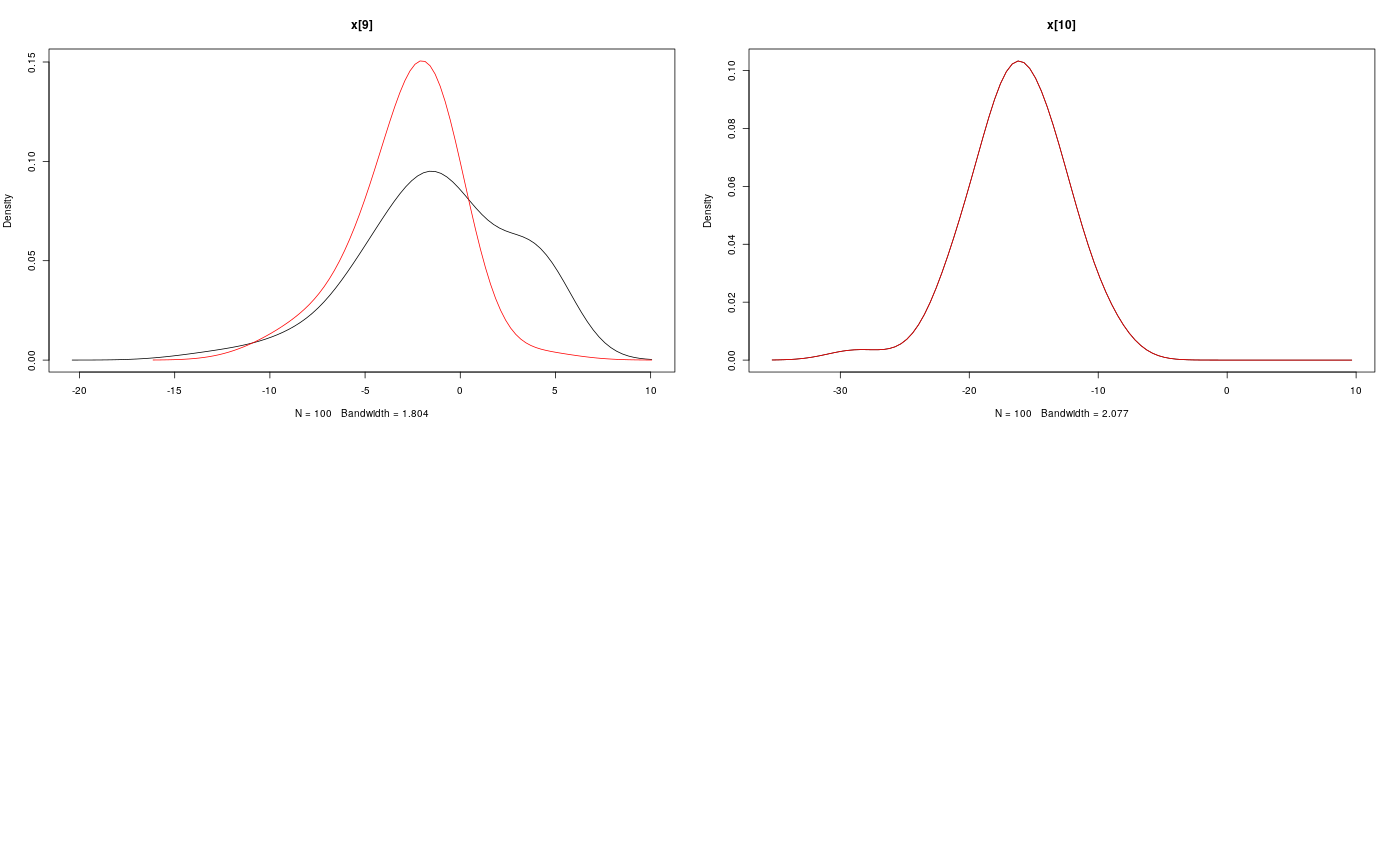
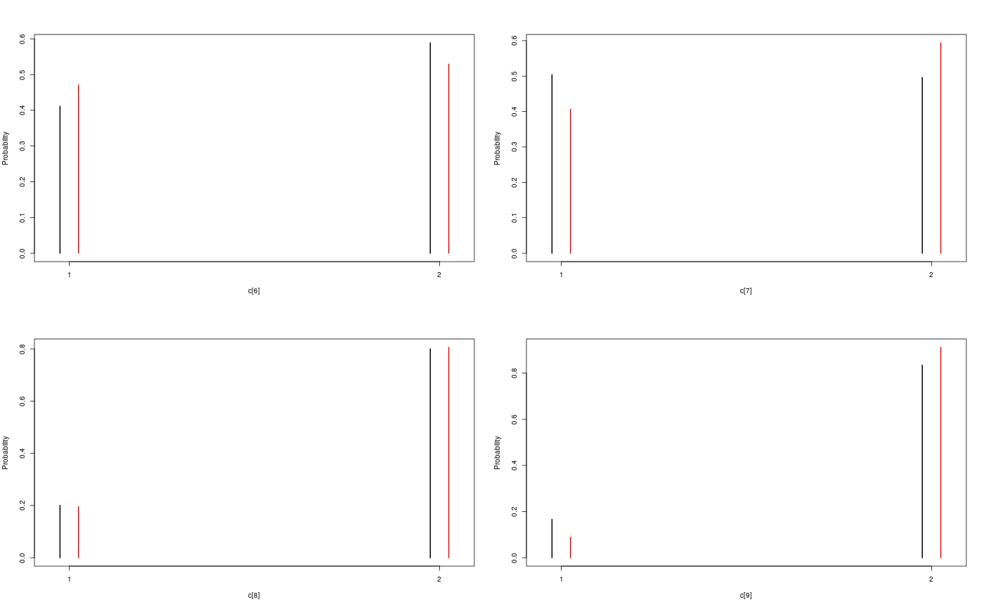
Examples

modelfile <- system.file('extdata', 'hmm.bug', package = 'rbiips')
stopifnot(nchar(modelfile) > 0)
cat(readLines(modelfile), sep = '\n')
#> var c_true[tmax], x_true[tmax], c[tmax], x[tmax], y[tmax]
#> 
#> data
#> {
#>   x_true[1] ~ dnorm(0, 1/5)
#>   y[1] ~ dnorm(x_true[1], exp(logtau_true))
#>   for (t in 2:tmax)
#>   {
#>     c_true[t] ~ dcat(p)
#>     x_true[t] ~ dnorm(0.5*x_true[t-1]+25*x_true[t-1]/(1+x_true[t-1]^2)+8*cos(1.2*(t-1)), ifelse(c_true[t]==1, 1/10, 1/100))
#>     y[t] ~ dnorm(x_true[t]/4, exp(logtau_true))
#>   }
#> }
#> 
#> model
#> {
#>   logtau ~ dunif(-3, 3)
#>   x[1] ~ dnorm(0, 1/5)
#>   y[1] ~ dnorm(x[1], exp(logtau))
#>   for (t in 2:tmax)
#>   {
#>     c[t] ~ dcat(p)
#>     x[t] ~ dnorm(0.5*x[t-1]+25*x[t-1]/(1+x[t-1]^2)+8*cos(1.2*(t-1)), ifelse(c[t]==1, 1/10, 1/100))
#>     y[t] ~ dnorm(x[t]/4, exp(logtau))
#>   }
#> }

data <- list(tmax = 10, p = c(.5, .5), logtau_true = log(1), logtau = log(1))
model <- biips_model(modelfile, data, sample_data = TRUE)
#> * Parsing model in: /home/adrien/Dropbox/workspace/rbiips/inst/extdata/hmm.bug
#> * Compiling data graph
#>   Declaring variables
#>   Resolving undeclared variables
#>   Allocating nodes
#>   Graph size: 169
#>   Sampling data
#>   Reading data back into data table
#> * Compiling model graph
#>   Declaring variables
#>   Resolving undeclared variables
#>   Allocating nodes
#>   Graph size: 180

n_part <- 100
out_smc <- biips_smc_samples(model, c('x', 'c[2:10]'), n_part, type = 'fs',
                             rs_thres = 0.5, rs_type = 'stratified')
#> * Assigning node samplers
#> * Running SMC forward sampler with 100 particles
#>   |--------------------------------------------------| 100%
#>   |**************************************************| 10 iterations in 0.00 s

#' Manipulate `smcarray.fsb.list` object
is.smcarray.fsb.list(out_smc)
#> [1] TRUE
names(out_smc)
#> [1] "c[2:10]"       "x"             "log_marg_like"
out_smc
#> c[2:10] filtering smcarray:
#> $mode
#> [1] 1 2 2 1 2 1 2 2 2
#> 
#> Marginalizing over: particle(100) 
#> 
#> c[2:10] smoothing smcarray:
#> $mode
#> [1] 1 2 2 1 2 2 2 2 2
#> 
#> Marginalizing over: particle(100) 
#> 
#> 
#> x filtering smcarray:
#> $mean
#>  [1]  -2.511252  -7.724433 -24.706784 -31.705386 -17.480945   4.353854
#>  [7]   6.651134  -8.015994  -1.153407 -16.278649
#> 
#> Marginalizing over: particle(100) 
#> 
#> x smoothing smcarray:
#> $mean
#>  [1]  -2.373479  -7.585363 -25.631439 -32.935665 -17.075466   4.024447
#>  [7]   5.548396  -7.289486  -2.802202 -16.278649
#> 
#> Marginalizing over: particle(100) 
#> 
#> 
#> Log-marginal likelihood:  -38.80216 
biips_diagnosis(out_smc)
#> * Diagnosis of variable: c[2:10] 
#>   Filtering: GOOD
#>   Smoothing: POOR
#>     The minimum effective sample size is too low: 12.59991 
#>     Estimates may be poor for some variables.
#>     You should increase the number of particles
#> .* Diagnosis of variable: x[1:10] 
#>   Filtering: GOOD
#>   Smoothing: POOR
#>     The minimum effective sample size is too low: 12.59991 
#>     Estimates may be poor for some variables.
#>     You should increase the number of particles
#> .
biips_summary(out_smc)
#> c[2:10] filtering smcarray:
#> $mode
#> [1] 1 2 2 1 2 1 2 2 2
#> 
#> Marginalizing over: particle(100) 
#> 
#> c[2:10] smoothing smcarray:
#> $mode
#> [1] 1 2 2 1 2 2 2 2 2
#> 
#> Marginalizing over: particle(100) 
#> 
#> 
#> x filtering smcarray:
#> $mean
#>  [1]  -2.511252  -7.724433 -24.706784 -31.705386 -17.480945   4.353854
#>  [7]   6.651134  -8.015994  -1.153407 -16.278649
#> 
#> Marginalizing over: particle(100) 
#> 
#> x smoothing smcarray:
#> $mean
#>  [1]  -2.373479  -7.585363 -25.631439 -32.935665 -17.075466   4.024447
#>  [7]   5.548396  -7.289486  -2.802202 -16.278649
#> 
#> Marginalizing over: particle(100) 
#> 
#> 

#' Manipulate `smcarray.fsb` object
is.smcarray.fsb(out_smc$x)
#> [1] TRUE
names(out_smc$x)
#> [1] "f" "s"
out_smc$x
#> filtering smcarray:
#> $mean
#>  [1]  -2.511252  -7.724433 -24.706784 -31.705386 -17.480945   4.353854
#>  [7]   6.651134  -8.015994  -1.153407 -16.278649
#> 
#> Marginalizing over: particle(100) 
#> 
#> smoothing smcarray:
#> $mean
#>  [1]  -2.373479  -7.585363 -25.631439 -32.935665 -17.075466   4.024447
#>  [7]   5.548396  -7.289486  -2.802202 -16.278649
#> 
#> Marginalizing over: particle(100) 
#> 
biips_diagnosis(out_smc$x)
#> * Diagnosis of variable: x[1:10] 
#>   Filtering: GOOD
#>   Smoothing: POOR
#>     The minimum effective sample size is too low: 12.59991 
#>     Estimates may be poor for some variables.
#>     You should increase the number of particles
#> .
summ_smc_x <- biips_summary(out_smc$x, order = 2, probs = c(.025, .975))
summ_smc_x
#> filtering smcarray:
#> $mean
#>  [1]  -2.511252  -7.724433 -24.706784 -31.705386 -17.480945   4.353854
#>  [7]   6.651134  -8.015994  -1.153407 -16.278649
#> 
#> $var
#>  [1]  0.7626423 10.4465326 19.8756192 11.9907475 10.4664837 15.7309246
#>  [7] 19.0697822 10.9846480 15.8809271 12.6805319
#> 
#> $probs
#> [1] 0.025 0.975
#> 
#> $quant
#> $quant$`0.025`
#>  [1]  -4.082389 -15.018010 -32.776464 -38.004680 -24.175178  -1.536774
#>  [7]  -4.761837 -12.725714 -11.380153 -23.187816
#> 
#> $quant$`0.975`
#>  [1]  -0.7822667  -3.3452161 -14.8996768 -23.9440440 -11.5875788  12.0310370
#>  [7]  14.1227257  -1.0294242   4.4873749  -8.8020497
#> 
#> 
#> Marginalizing over: particle(100) 
#> 
#> smoothing smcarray:
#> $mean
#>  [1]  -2.373479  -7.585363 -25.631439 -32.935665 -17.075466   4.024447
#>  [7]   5.548396  -7.289486  -2.802202 -16.278649
#> 
#> $var
#>  [1]  0.6444075 14.3199922 14.6778972  5.6757351  9.7754211 11.5837880
#>  [7] 20.0829903  7.2940514  6.1104302 12.6805319
#> 
#> $probs
#> [1] 0.025 0.975
#> 
#> $quant
#> $quant$`0.025`
#>  [1]  -4.045283 -14.777315 -31.924168 -37.602509 -22.773549  -2.222205
#>  [7]  -3.401456 -12.748046  -7.957866 -23.187816
#> 
#> $quant$`0.975`
#>  [1]  -1.0292148  -2.4584248 -16.5758012 -28.8476022 -11.4408993   9.4616870
#>  [7]  13.3746680  -2.5775357   0.8573436  -8.8020497
#> 
#> 
#> Marginalizing over: particle(100) 
#> 
dens_smc_x <- biips_density(out_smc$x, bw = 'nrd0', adjust = 1, n = 100)
par(mfrow = c(2, 2))
plot(dens_smc_x)

is.smcarray.fsb(out_smc[['c[2:10]']])
#> [1] TRUE
names(out_smc[['c[2:10]']])
#> [1] "f" "s"
out_smc[['c[2:10]']]
#> filtering smcarray:
#> $mode
#> [1] 1 2 2 1 2 1 2 2 2
#> 
#> Marginalizing over: particle(100) 
#> 
#> smoothing smcarray:
#> $mode
#> [1] 1 2 2 1 2 2 2 2 2
#> 
#> Marginalizing over: particle(100) 
#> 
biips_diagnosis(out_smc[['c[2:10]']])
#> * Diagnosis of variable: c[2:10] 
#>   Filtering: GOOD
#>   Smoothing: POOR
#>     The minimum effective sample size is too low: 12.59991 
#>     Estimates may be poor for some variables.
#>     You should increase the number of particles
#> .
summ_smc_c <- biips_summary(out_smc[['c[2:10]']])
summ_smc_c
#> filtering smcarray:
#> $mode
#> [1] 1 2 2 1 2 1 2 2 2
#> 
#> Marginalizing over: particle(100) 
#> 
#> smoothing smcarray:
#> $mode
#> [1] 1 2 2 1 2 2 2 2 2
#> 
#> Marginalizing over: particle(100) 
#> 
table_smc_c <- biips_table(out_smc[['c[2:10]']])
par(mfrow = c(2, 2))
plot(table_smc_c)

#' Manipulate `smcarray` object
is.smcarray(out_smc$x$f)
#> [1] TRUE
names(out_smc$x$f)
#>  [1] "values"       "weights"      "ess"          "discrete"     "iterations"  
#>  [6] "conditionals" "name"         "lower"        "upper"        "type"        
out_smc$x$f
#> smcarray:
#> $mean
#>  [1]  -2.511252  -7.724433 -24.706784 -31.705386 -17.480945   4.353854
#>  [7]   6.651134  -8.015994  -1.153407 -16.278649
#> 
#> Marginalizing over: particle(100) 
out_smc$x$s
#> smcarray:
#> $mean
#>  [1]  -2.373479  -7.585363 -25.631439 -32.935665 -17.075466   4.024447
#>  [7]   5.548396  -7.289486  -2.802202 -16.278649
#> 
#> Marginalizing over: particle(100) 
biips_diagnosis(out_smc$x$f)
#> * Diagnosis of variable: x[1:10] 
#>   Filtering: GOOD
biips_diagnosis(out_smc$x$s)
#> * Diagnosis of variable: x[1:10] 
#>   Smoothing: POOR
#>     The minimum effective sample size is too low: 12.59991 
#>     Estimates may be poor for some variables.
#>     You should increase the number of particles
#> .
biips_summary(out_smc$x$f)
#> smcarray:
#> $mean
#>  [1]  -2.511252  -7.724433 -24.706784 -31.705386 -17.480945   4.353854
#>  [7]   6.651134  -8.015994  -1.153407 -16.278649
#> 
#> Marginalizing over: particle(100) 
biips_summary(out_smc$x$s)
#> smcarray:
#> $mean
#>  [1]  -2.373479  -7.585363 -25.631439 -32.935665 -17.075466   4.024447
#>  [7]   5.548396  -7.289486  -2.802202 -16.278649
#> 
#> Marginalizing over: particle(100) 
par(mfrow = c(2, 2))
plot(biips_density(out_smc$x$f))
par(mfrow = c(2, 2))
plot(biips_density(out_smc$x$s))

par(mfrow = c(2, 2))
plot(biips_table(out_smc[['c[2:10]']]$f))
par(mfrow = c(2, 2))
plot(biips_table(out_smc[['c[2:10]']]$s))