This is a quick demo of rbiips main functions.

Disclaimer: for speed of execution, we use very few particles and MCMC iterations in this vignette. As such, the results are not representative of the perforance of SMC and particle MCMC methods.

set.seed(0)
library(rbiips)

Add custom functions and distributions to BUGS language

Add custom function f

f_dim <- function(x_dim, t_dim) {
  # Check dimensions of the input and return dimension of the output of function f
  stopifnot(prod(x_dim) == 1, prod(t_dim) == 1)
  x_dim
}
f_eval <- function(x, t) {
  # Evaluate function f
  0.5 * x + 25 * x/(1 + x^2) + 8 * cos(1.2 * t)
}
biips_add_function('f', 2, f_dim, f_eval)

## * Added function f

Add custom sampling distribution dMN

dMN_dim <- function(mu_dim, Sig_dim) {
  # Check dimensions of the input and return dimension of the output of
  # distribution dMN
  stopifnot(prod(mu_dim) == mu_dim[1], length(Sig_dim) == 2, mu_dim[1] == Sig_dim)
  mu_dim
}
dMN_sample <- function(mu, Sig) {
  # Draw a sample of distribution dMN
  mu + t(chol(Sig)) %*% rnorm(length(mu))
}
biips_add_distribution('dMN', 2, dMN_dim, dMN_sample)

## * Added distribution dMN

Compile model

modelfile <- system.file('extdata', 'hmm_f.bug', package = 'rbiips')
stopifnot(nchar(modelfile) > 0)
cat(readLines(modelfile), sep = '\n')

## var c_true[tmax], x_true[tmax], c[tmax], x[tmax], y[tmax]
## 
## data
## {
##   x_true[1] ~ dnorm(0, 1/5)
##   y[1] ~ dnorm(x_true[1], exp(logtau_true))
##   for (t in 2:tmax)
##   {
##     c_true[t] ~ dcat(p)
##     x_true[t] ~ dnorm(f(x_true[t-1], t-1), ifelse(c_true[t]==1, 1/10, 1/100))
##     y[t] ~ dnorm(x_true[t]/4, exp(logtau_true))
##   }
## }
## 
## model
## {
##   logtau ~ dunif(-3, 3)
##   x[1] ~ dnorm(0, 1/5)
##   y[1] ~ dnorm(x[1], exp(logtau))
##   for (t in 2:tmax)
##   {
##     c[t] ~ dcat(p)
##     x[t] ~ dnorm(f(x[t-1], t-1), ifelse(c[t]==1, 1/10, 1/100))
##     y[t] ~ dnorm(x[t]/4, exp(logtau))
##   }
## }

tmax <- 10
data_ <- list(tmax = tmax, p = c(.5, .5), logtau_true = log(1), logtau = log(1))
model <- biips_model(modelfile, data_, sample_data = TRUE)

## * Parsing model in: /home/adrien/R/x86_64-pc-linux-gnu-library/3.4/rbiips/extdata/hmm_f.bug
## * Compiling data graph
##   Declaring variables
##   Resolving undeclared variables
##   Allocating nodes
##   Graph size: 94
##   Sampling data
##   Reading data back into data table
## * Compiling model graph
##   Declaring variables
##   Resolving undeclared variables
##   Allocating nodes
##   Graph size: 105

data_ = model$data()

SMC algorithm

n_part <- 100
out_smc <- biips_smc_samples(model, c('x', 'c[2:10]', 'x[5]', 'c[5]'), 
                             n_part, type = 'fs',
                             rs_thres = 0.5, rs_type = 'stratified')

## * Assigning node samplers
## * Running SMC forward sampler with 100 particles
##   |--------------------------------------------------| 100%
##   |**************************************************| 10 iterations in 0.04 s

biips_diagnosis(out_smc)

## * Diagnosis of variable: c[2:10] 
##   Filtering: GOOD
##   Smoothing: POOR
##     The minimum effective sample size is too low: 27.97195 
##     Estimates may be poor for some variables.
##     You should increase the number of particles
## .* Diagnosis of variable: c[5] 
##   Filtering: GOOD
##   Smoothing: POOR
##     The minimum effective sample size is too low: 27.97195 
##     Estimates may be poor for some variables.
##     You should increase the number of particles
## .* Diagnosis of variable: x[1:10] 
##   Filtering: GOOD
##   Smoothing: POOR
##     The minimum effective sample size is too low: 27.97195 
##     Estimates may be poor for some variables.
##     You should increase the number of particles
## .* Diagnosis of variable: x[5] 
##   Filtering: GOOD
##   Smoothing: POOR
##     The minimum effective sample size is too low: 27.97195 
##     Estimates may be poor for some variables.
##     You should increase the number of particles
## .

summ_smc <- biips_summary(out_smc, probs=c(0.025, 0.975))

par(mfrow = c(2, 2), bty='l')

matplot(do.call(cbind, summ_smc$x$f$quant), 
        type='n', xlab='t', ylab='x[t]')
lines(summ_smc$x$f$mean)
matlines(do.call(cbind, summ_smc$x$f$quant), col=1, lty=2)
lines(summ_smc$x$s$mean, col=2)
matlines(do.call(cbind, summ_smc$x$s$quant), col=2, lty=2)
lines(data_$x_true, col=3)
legend('topleft', 
       leg=c('SMC filtering estimate',
             'SMC smoothing estimate', 'true'),
       col=1:3, lty=1, bty='n')

matplot(c(1,tmax), c(0,4), type='n', xlab='t', ylab='c[t]==1', yaxt='n')
lines(2:tmax, 2+summ_smc[['c[2:10]']]$f$mode, type='S')
lines(2:tmax, .5+summ_smc[['c[2:10]']]$s$mode, type='S', col=2)
lines(-1+data_$c_true, type='S', col=3)
legend('topleft', 
       leg=c('SMC filtering mode',
             'SMC smoothing mode', 'true'),
       col=1:3, lty=1, bty='n')

plot(biips_density(out_smc[['x[5]']]))
abline(v=data_$x_true[5], col=3)

plot(biips_table(out_smc[['c[5]']]))
points(data_$c_true[5], 0, col=3, pch=17)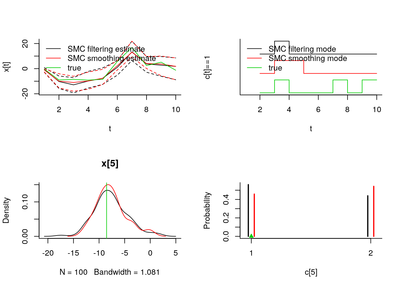

PIMH algorithm

n_part <- 50
obj_pimh <- biips_pimh_init(model, c('x', 'c[2:10]', 'x[5]', 'c[5]'))  # Initialize

## * Initializing PIMH

out_pimh_burn <- biips_pimh_update(obj_pimh, 100, n_part)  # Burn-in

## * Updating PIMH with 50 particles
##   |--------------------------------------------------| 100%
##   |**************************************************| 100 iterations in 1.87 s

out_pimh <- biips_pimh_samples(obj_pimh, 100, n_part)  # Samples

## * Generating PIMH samples with 50 particles
##   |--------------------------------------------------| 100%
##   |**************************************************| 100 iterations in 1.85 s

summ_pimh <- biips_summary(out_pimh, probs=c(0.025, 0.975))

par(mfrow = c(2, 1), bty='l')

plot(c(out_pimh_burn$log_marg_like, out_pimh$log_marg_like),
     type = 'l', xlab = 'PIMH iteration', ylab = 'log p(y)')

plot(101:200, c(out_pimh[['x[5]']]),
     type = 'l', xlab = 'PIMH iteration', ylab = 'x[5]')
abline(h=data_$x_true[5], col = 3)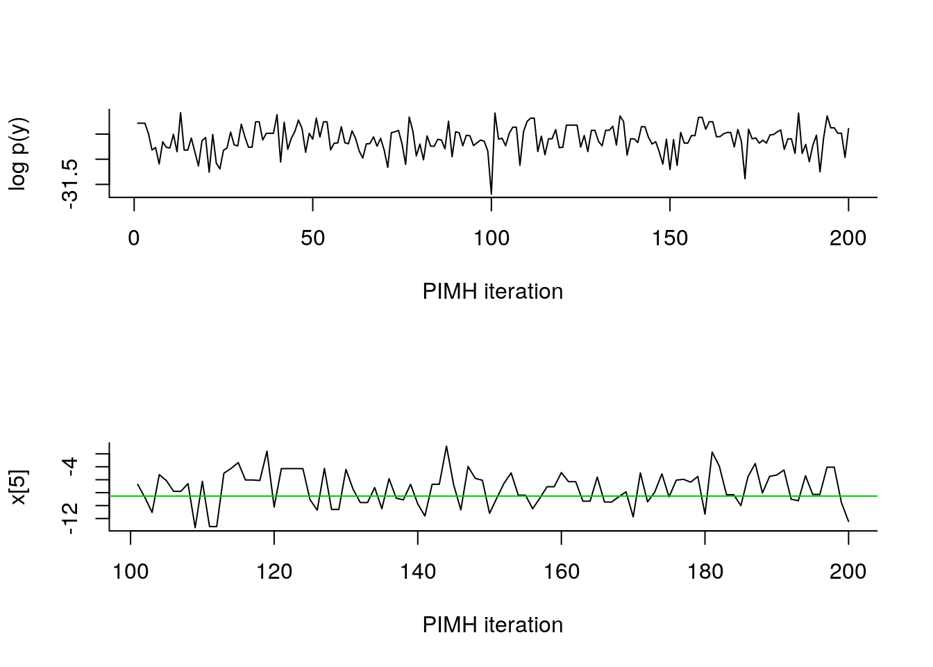

par(mfrow = c(2, 2), bty='l')

matplot(do.call(cbind, summ_pimh$x$quant), 
        type='n', xlab='t', ylab='x[t]')
lines(summ_pimh$x$mean)
matlines(do.call(cbind, summ_pimh$x$quant), col=1, lty=2)
lines(data_$x_true, col=3)
legend('topleft', 
       leg=c('PIMH estimate', 'true'),
       col=c(1,3), lty=1, bty='n')

matplot(c(1,tmax), c(0,2.5), type='n', xlab='t', ylab='c[t]==1', yaxt='n')
lines(2:tmax, .5+summ_pimh[['c[2:10]']]$mode, type='S')
lines(-1+data_$c_true, type='S', col=3)
legend('topleft', 
       leg=c('PIMH mode', 'true'),
       col=c(1,3), lty=1, bty='n')

plot(biips_density(out_pimh[['x[5]']]))
abline(v=data_$x_true[5], col=3)

plot(biips_table(out_pimh[['c[5]']]))
points(data_$c_true[5], 0, col=3, pch=17)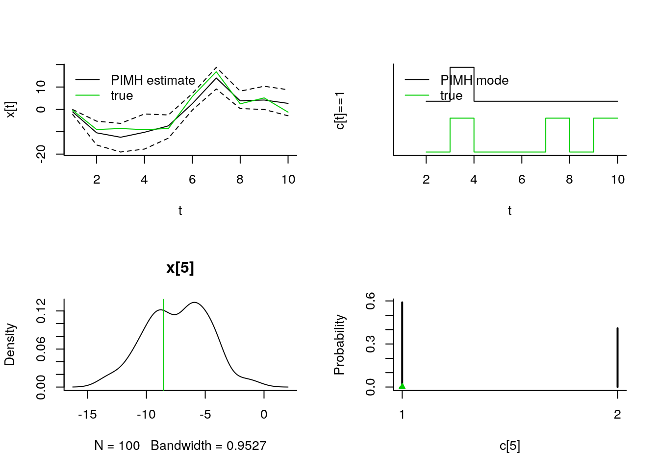

SMC sensitivity analysis

n_part <- 50
logtau_val <- -10:10
out_sens <- biips_smc_sensitivity(model, list(logtau = logtau_val), n_part)

## * Analyzing sensitivity with 50 particles
##   |--------------------------------------------------| 100%
##   |**************************************************| 21 iterations in 0.32 s

par(mfrow = c(2,1), bty='l')
plot(logtau_val, out_sens$log_marg_like, type='l',
     xlab = 'logtau', ylab = 'log p(y | logtau)')
abline(v=data_$logtau_true, col=3)

plot(logtau_val, out_sens$log_marg_like_pen, type='l',
     xlab = 'logtau', ylab = 'log p(y, logtau)')
abline(v=data_$logtau_true, col=3)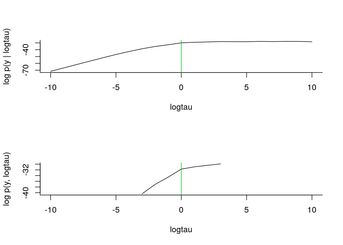

PMMH algorithm

data_ <- list(tmax = 10, p = c(.5, .5), logtau_true = log(1))
model <- biips_model(modelfile, data_)

## * Parsing model in: /home/adrien/R/x86_64-pc-linux-gnu-library/3.4/rbiips/extdata/hmm_f.bug
## * Compiling data graph
##   Declaring variables
##   Resolving undeclared variables
##   Allocating nodes
##   Graph size: 93
##   Sampling data
##   Reading data back into data table
## * Compiling model graph
##   Declaring variables
##   Resolving undeclared variables
##   Allocating nodes
##   Graph size: 105

data_ <- model$data()

n_part <- 50
n_burn <- 100
n_iter <- 100
obj_pmmh <- biips_pmmh_init(model, 'logtau', 
                            latent_names = c('x', 'c[2:10]', 'x[5]', 'c[5]'),
                            inits = list(logtau = -1))  # Initialize

## * Initializing PMMH

out_pmmh_burn <- biips_pmmh_update(obj_pmmh, n_burn, n_part)  # Burn-in

## * Adapting PMMH with 50 particles
##   |--------------------------------------------------| 100%
##   |++++++++++++++++++++++++++++++++++++++++++++++++++| 100 iterations in 1.88 s

out_pmmh <- biips_pmmh_samples(obj_pmmh, n_iter, n_part, thin = 1)  # Samples

## * Generating 100 PMMH samples with 50 particles
##   |--------------------------------------------------| 100%
##   |**************************************************| 100 iterations in 1.67 s

summ_pmmh <- biips_summary(out_pmmh, probs=c(.025, 0.975))

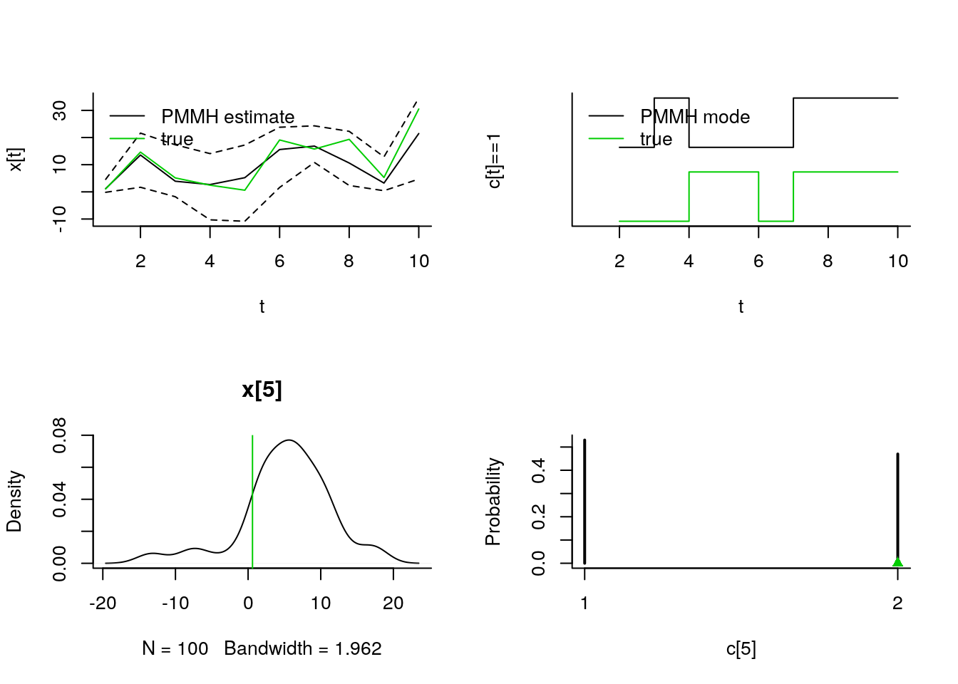
par(mfrow = c(2, 2), bty='l')

plot(c(out_pmmh_burn$log_marg_like_pen, out_pimh$log_marg_like_pen),
     type = 'l', xlab = 'PMMH iteration', ylab = 'log p(y, logtau)')

plot(n_burn+(1:n_iter), c(out_pmmh$logtau),
     type = 'l', xlab = 'PMMH iteration', ylab = 'logtau')
abline(h=data_$logtau_true, col = 3)

plot(biips_density(out_pmmh$logtau))
abline(v=data_$logtau_true, col=3)

biips_hist(out_pmmh$logtau)
abline(v=data_$logtau_true, col=3)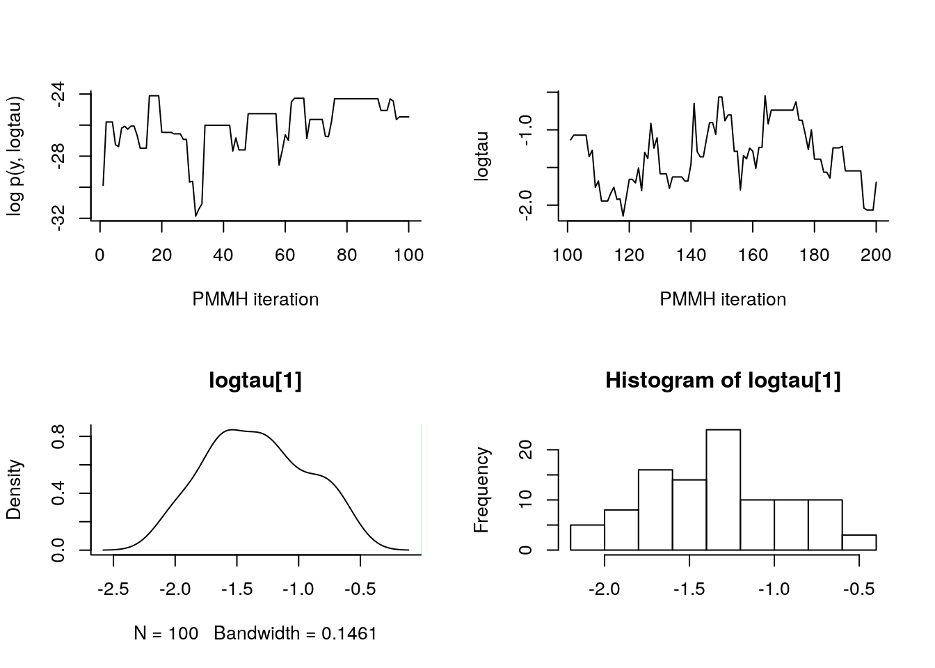

matplot(do.call(cbind, summ_pmmh$x$quant), 
        type='n', xlab='t', ylab='x[t]')
lines(summ_pmmh$x$mean)
matlines(do.call(cbind, summ_pmmh$x$quant), lty=2, col=1)
lines(data_$x_true, col=3)
legend('topleft', 
       leg=c('PMMH estimate', 'true'),
       col=c(1,3), lty=1, bty='n')

matplot(c(1,tmax), c(0,2.5), type='n', xlab='t', ylab='c[t]==1', yaxt='n')
lines(2:tmax, .5+summ_pmmh[['c[2:10]']]$mode, type='S')
lines(-1+data_$c_true, type='S', col=3)
legend('topleft', 
       leg=c('PMMH mode', 'true'),
       col=c(1,3), lty=1, bty='n')

plot(biips_density(out_pmmh[['x[5]']]))
abline(v=data_$x_true[5], col=3)

plot(biips_table(out_pmmh[['c[5]']]))
points(data_$c_true[5], 0, col=3, pch=17)

rbiips demo

Adrien Todeschini, François Caron