This vignette gathers the examples used in the rbiips reference manual.
set.seed(0)
library(rbiips)
Add custom functions and distributions to BUGS language
Add custom function f
f_dim <- function(x_dim, t_dim) {
  # Check dimensions of the input and return dimension of the output of function f
  stopifnot(prod(x_dim) == 1, prod(t_dim) == 1)
  x_dim
}
f_eval <- function(x, t) {
  # Evaluate function f
  0.5 * x + 25 * x/(1 + x^2) + 8 * cos(1.2 * t)
}
biips_add_function('f', 2, f_dim, f_eval)
## * Added function fAdd custom sampling distribution dMN
dMN_dim <- function(mu_dim, Sig_dim) {
  # Check dimensions of the input and return dimension of the output of
  # distribution dMN
  stopifnot(prod(mu_dim) == mu_dim[1], length(Sig_dim) == 2, mu_dim[1] == Sig_dim)
  mu_dim
}
dMN_sample <- function(mu, Sig) {
  # Draw a sample of distribution dMN
  mu + t(chol(Sig)) %*% rnorm(length(mu))
}
biips_add_distribution('dMN', 2, dMN_dim, dMN_sample)
## * Added distribution dMNCompile model
modelfile <- system.file('extdata', 'hmm_f.bug', package = 'rbiips')
stopifnot(nchar(modelfile) > 0)
cat(readLines(modelfile), sep = '\n')
## var c_true[tmax], x_true[tmax], c[tmax], x[tmax], y[tmax]
##
## data
## {
## x_true[1] ~ dnorm(0, 1/5)
## y[1] ~ dnorm(x_true[1], exp(logtau_true))
## for (t in 2:tmax)
## {
## c_true[t] ~ dcat(p)
## x_true[t] ~ dnorm(f(x_true[t-1], t-1), ifelse(c_true[t]==1, 1/10, 1/100))
## y[t] ~ dnorm(x_true[t]/4, exp(logtau_true))
## }
## }
##
## model
## {
## logtau ~ dunif(-3, 3)
## x[1] ~ dnorm(0, 1/5)
## y[1] ~ dnorm(x[1], exp(logtau))
## for (t in 2:tmax)
## {
## c[t] ~ dcat(p)
## x[t] ~ dnorm(f(x[t-1], t-1), ifelse(c[t]==1, 1/10, 1/100))
## y[t] ~ dnorm(x[t]/4, exp(logtau))
## }
## }data <- list(tmax = 10, p = c(.5, .5), logtau_true = log(1), logtau = log(1))
model <- biips_model(modelfile, data, sample_data = TRUE)## * Parsing model in: /home/adrien/R/x86_64-pc-linux-gnu-library/3.4/rbiips/extdata/hmm_f.bug
## * Compiling data graph
## Declaring variables
## Resolving undeclared variables
## Allocating nodes
## Graph size: 94
## Sampling data
## Reading data back into data table
## * Compiling model graph
## Declaring variables
## Resolving undeclared variables
## Allocating nodes
## Graph size: 105# rm(model)
#
# tmax <- 10
# p <- c(.5, .5)
# logtau_true <- log(1)
# logtau <- logtau_true
#
# datanames <- c('tmax', 'p', 'logtau_true', 'logtau')
# model <- biips_model(modelfile, datanames, sample_data = TRUE)
is.biips(model)## [1] TRUEprint(model)## Biips model:
##
## var c_true[tmax], x_true[tmax], c[tmax], x[tmax], y[tmax]
##
## data
## {
##   x_true[1] ~ dnorm(0, 1/5)
##   y[1] ~ dnorm(x_true[1], exp(logtau_true))
##   for (t in 2:tmax)
##   {
##     c_true[t] ~ dcat(p)
##     x_true[t] ~ dnorm(f(x_true[t-1], t-1), ifelse(c_true[t]==1, 1/10, 1/100))
##     y[t] ~ dnorm(x_true[t]/4, exp(logtau_true))
##   }
## }
##
## model
## {
##   logtau ~ dunif(-3, 3)
##   x[1] ~ dnorm(0, 1/5)
##   y[1] ~ dnorm(x[1], exp(logtau))
##   for (t in 2:tmax)
##   {
##     c[t] ~ dcat(p)
##     x[t] ~ dnorm(f(x[t-1], t-1), ifelse(c[t]==1, 1/10, 1/100))
##     y[t] ~ dnorm(x[t]/4, exp(logtau))
##   }
## }
##
##
## Fully observed variables:
## logtau logtau_true p tmax x_true y
##
## Partially observed variables:
## c_truemodel$data()## $c_true
## [1] NA 1 1 2 1 1 1 2 1 2
##
## $logtau
## [1] 0
##
## $logtau_true
## [1] 0
##
## $p
## [1] 0.5 0.5
##
## $tmax
## [1] 10
##
## $x_true
## [1] -0.4169979 -9.0124859 -8.5502201 -9.0831363 -8.5299593 5.7598874
## [7] 16.8533731 2.4722914 5.1386416 -1.2379888
##
## $y
## [1] -1.0915320 -2.8456504 -2.9185889 -1.7675427 -1.9918904 0.2540241
## [7] 3.4715740 0.5880222 1.0806876 0.1869324variable.names(model)## [1] "c" "c_true" "logtau" "logtau_true" "p"
## [6] "tmax" "x" "x_true" "y"biips_variable_names(model)## [1] "c" "c_true" "logtau" "logtau_true" "p"
## [6] "tmax" "x" "x_true" "y"biips_nodes(model)## id name type observed discrete
## 1 0 c_true[2] const TRUE TRUE
## 2 1 c_true[3] const TRUE TRUE
## 3 2 c_true[4] const TRUE TRUE
## 4 3 c_true[5] const TRUE TRUE
## 5 4 c_true[6] const TRUE TRUE
## 6 5 c_true[7] const TRUE TRUE
## 7 6 c_true[8] const TRUE TRUE
## 8 7 c_true[9] const TRUE TRUE
## 9 8 c_true[10] const TRUE TRUE
## 10 9 logtau_true const TRUE TRUE
## 11 10 p const TRUE FALSE
## 12 11 tmax const TRUE TRUE
## 13 12 x_true const TRUE FALSE
## 14 13 3 const TRUE TRUE
## 15 14 (-3) logic TRUE TRUE
## 16 15 logtau stoch TRUE FALSE
## 17 21 (exp(logtau)) logic TRUE FALSE
## 18 16 0 const TRUE TRUE
## 19 17 1 const TRUE TRUE
## 20 38 (3-1) logic TRUE TRUE
## 21 18 5 const TRUE TRUE
## 22 19 (1/5) logic TRUE FALSE
## 23 54 (5-1) logic TRUE TRUE
## 24 20 x[1] stoch FALSE FALSE
## 25 22 y[1] stoch TRUE FALSE
## 26 23 c[2] stoch FALSE TRUE
## 27 27 (c[2]==1) logic FALSE TRUE
## 28 24 2 const TRUE TRUE
## 29 25 (2-1) logic TRUE TRUE
## 30 26 (f(x[1],(2-1))) logic FALSE FALSE
## 31 28 10 const TRUE TRUE
## 32 29 (1/10) logic TRUE FALSE
## 33 98 (10-1) logic TRUE TRUE
## 34 30 100 const TRUE TRUE
## 35 31 (1/100) logic TRUE FALSE
## 36 32 (ifelse((c[2]==1),(1/10),(1/100))) logic FALSE FALSE
## 37 33 x[2] stoch FALSE FALSE
## 38 39 (f(x[2],(3-1))) logic FALSE FALSE
## 39 34 4 const TRUE TRUE
## 40 35 (x[2]/4) logic FALSE FALSE
## 41 36 y[2] stoch TRUE FALSE
## 42 46 (4-1) logic TRUE TRUE
## 43 37 c[3] stoch FALSE TRUE
## 44 40 (c[3]==1) logic FALSE TRUE
## 45 41 (ifelse((c[3]==1),(1/10),(1/100))) logic FALSE FALSE
## 46 42 x[3] stoch FALSE FALSE
## 47 43 (x[3]/4) logic FALSE FALSE
## 48 44 y[3] stoch TRUE FALSE
## 49 47 (f(x[3],(4-1))) logic FALSE FALSE
## 50 45 c[4] stoch FALSE TRUE
## 51 48 (c[4]==1) logic FALSE TRUE
## 52 49 (ifelse((c[4]==1),(1/10),(1/100))) logic FALSE FALSE
## 53 50 x[4] stoch FALSE FALSE
## 54 51 (x[4]/4) logic FALSE FALSE
## 55 52 y[4] stoch TRUE FALSE
## 56 55 (f(x[4],(5-1))) logic FALSE FALSE
## 57 53 c[5] stoch FALSE TRUE
## 58 56 (c[5]==1) logic FALSE TRUE
## 59 57 (ifelse((c[5]==1),(1/10),(1/100))) logic FALSE FALSE
## 60 58 x[5] stoch FALSE FALSE
## 61 59 (x[5]/4) logic FALSE FALSE
## 62 60 y[5] stoch TRUE FALSE
## 63 61 c[6] stoch FALSE TRUE
## 64 65 (c[6]==1) logic FALSE TRUE
## 65 66 (ifelse((c[6]==1),(1/10),(1/100))) logic FALSE FALSE
## 66 62 6 const TRUE TRUE
## 67 63 (6-1) logic TRUE TRUE
## 68 64 (f(x[5],(6-1))) logic FALSE FALSE
## 69 67 x[6] stoch FALSE FALSE
## 70 68 (x[6]/4) logic FALSE FALSE
## 71 69 y[6] stoch TRUE FALSE
## 72 70 c[7] stoch FALSE TRUE
## 73 74 (c[7]==1) logic FALSE TRUE
## 74 75 (ifelse((c[7]==1),(1/10),(1/100))) logic FALSE FALSE
## 75 71 7 const TRUE TRUE
## 76 72 (7-1) logic TRUE TRUE
## 77 73 (f(x[6],(7-1))) logic FALSE FALSE
## 78 76 x[7] stoch FALSE FALSE
## 79 77 (x[7]/4) logic FALSE FALSE
## 80 78 y[7] stoch TRUE FALSE
## 81 79 c[8] stoch FALSE TRUE
## 82 83 (c[8]==1) logic FALSE TRUE
## 83 84 (ifelse((c[8]==1),(1/10),(1/100))) logic FALSE FALSE
## 84 80 8 const TRUE TRUE
## 85 81 (8-1) logic TRUE TRUE
## 86 82 (f(x[7],(8-1))) logic FALSE FALSE
## 87 85 x[8] stoch FALSE FALSE
## 88 86 (x[8]/4) logic FALSE FALSE
## 89 87 y[8] stoch TRUE FALSE
## 90 88 c[9] stoch FALSE TRUE
## 91 92 (c[9]==1) logic FALSE TRUE
## 92 93 (ifelse((c[9]==1),(1/10),(1/100))) logic FALSE FALSE
## 93 89 9 const TRUE TRUE
## 94 90 (9-1) logic TRUE TRUE
## 95 91 (f(x[8],(9-1))) logic FALSE FALSE
## 96 94 x[9] stoch FALSE FALSE
## 97 95 (x[9]/4) logic FALSE FALSE
## 98 96 y[9] stoch TRUE FALSE
## 99 99 (f(x[9],(10-1))) logic FALSE FALSE
## 100 97 c[10] stoch FALSE TRUE
## 101 100 (c[10]==1) logic FALSE TRUE
## 102 101 (ifelse((c[10]==1),(1/10),(1/100))) logic FALSE FALSE
## 103 102 x[10] stoch FALSE FALSE
## 104 103 (x[10]/4) logic FALSE FALSE
## 105 104 y[10] stoch TRUE FALSE# dotfile <- 'hmm.dot'
# biips_print_dot(model, dotfile)
# cat(readLines(dotfile), sep = '\n')SMC algorithm
biips_build_sampler(model, proposal = 'prior')## * Assigning node samplersbiips_nodes(model, type = 'stoch', observed = FALSE)## id name type observed discrete iteration sampler
## 24 20 x[1] stoch FALSE FALSE 0 Prior
## 26 23 c[2] stoch FALSE TRUE 1 Prior
## 37 33 x[2] stoch FALSE FALSE 1 Prior
## 43 37 c[3] stoch FALSE TRUE 2 Prior
## 46 42 x[3] stoch FALSE FALSE 2 Prior
## 50 45 c[4] stoch FALSE TRUE 3 Prior
## 53 50 x[4] stoch FALSE FALSE 3 Prior
## 57 53 c[5] stoch FALSE TRUE 4 Prior
## 60 58 x[5] stoch FALSE FALSE 4 Prior
## 63 61 c[6] stoch FALSE TRUE 5 Prior
## 69 67 x[6] stoch FALSE FALSE 5 Prior
## 72 70 c[7] stoch FALSE TRUE 6 Prior
## 78 76 x[7] stoch FALSE FALSE 6 Prior
## 81 79 c[8] stoch FALSE TRUE 7 Prior
## 87 85 x[8] stoch FALSE FALSE 7 Prior
## 90 88 c[9] stoch FALSE TRUE 8 Prior
## 96 94 x[9] stoch FALSE FALSE 8 Prior
## 100 97 c[10] stoch FALSE TRUE 9 Prior
## 103 102 x[10] stoch FALSE FALSE 9 Priorbiips_build_sampler(model, proposal = 'auto')## * Assigning node samplersbiips_nodes(model, type = 'stoch', observed = FALSE)## id name type observed discrete iteration
## 24 20 x[1] stoch FALSE FALSE 0
## 26 23 c[2] stoch FALSE TRUE 1
## 37 33 x[2] stoch FALSE FALSE 1
## 43 37 c[3] stoch FALSE TRUE 2
## 46 42 x[3] stoch FALSE FALSE 2
## 50 45 c[4] stoch FALSE TRUE 3
## 53 50 x[4] stoch FALSE FALSE 3
## 57 53 c[5] stoch FALSE TRUE 4
## 60 58 x[5] stoch FALSE FALSE 4
## 63 61 c[6] stoch FALSE TRUE 5
## 69 67 x[6] stoch FALSE FALSE 5
## 72 70 c[7] stoch FALSE TRUE 6
## 78 76 x[7] stoch FALSE FALSE 6
## 81 79 c[8] stoch FALSE TRUE 7
## 87 85 x[8] stoch FALSE FALSE 7
## 90 88 c[9] stoch FALSE TRUE 8
## 96 94 x[9] stoch FALSE FALSE 8
## 100 97 c[10] stoch FALSE TRUE 9
## 103 102 x[10] stoch FALSE FALSE 9
## sampler
## 24 ConjugateNormal_knownPrec
## 26 Prior
## 37 ConjugateNormal_knownPrec_linearMean
## 43 Prior
## 46 ConjugateNormal_knownPrec_linearMean
## 50 Prior
## 53 ConjugateNormal_knownPrec_linearMean
## 57 Prior
## 60 ConjugateNormal_knownPrec_linearMean
## 63 Prior
## 69 ConjugateNormal_knownPrec_linearMean
## 72 Prior
## 78 ConjugateNormal_knownPrec_linearMean
## 81 Prior
## 87 ConjugateNormal_knownPrec_linearMean
## 90 Prior
## 96 ConjugateNormal_knownPrec_linearMean
## 100 Prior
## 103 ConjugateNormal_knownPrec_linearMeann_part <- 100
out_smc <- biips_smc_samples(model, c('x', 'c[2:10]'), n_part, type = 'fs',
rs_thres = 0.5, rs_type = 'stratified')## * Running SMC forward sampler with 100 particles
## |--------------------------------------------------| 100%
## |**************************************************| 10 iterations in 0.03 sManipulate smcarray.fsb.list object
is.smcarray.fsb.list(out_smc)## [1] TRUEnames(out_smc)## [1] "c[2:10]" "x" "log_marg_like"out_smc## c[2:10] filtering smcarray:
## $mode
## [1] 1 1 2 1 1 1 1 1 1
##
## Marginalizing over: particle(100)
##
## c[2:10] smoothing smcarray:
## $mode
## [1] 1 1 2 2 1 1 1 1 1
##
## Marginalizing over: particle(100)
##
##
## x filtering smcarray:
## $mean
## [1] -0.8185253 -10.2517614 -12.8818052 -9.8706867 -7.6815614
## [6] 1.0595768 13.3149162 3.7425798 2.7491513 1.8215615
##
## Marginalizing over: particle(100)
##
## x smoothing smcarray:
## $mean
## [1] -1.075535 -9.946487 -11.013764 -9.784847 -7.637991 2.329093
## [7] 13.109354 4.027466 3.708989 1.821561
##
## Marginalizing over: particle(100)
##
##
## Log-marginal likelihood: -30.7798biips_diagnosis(out_smc)## * Diagnosis of variable: c[2:10]
## Filtering: GOOD
## Smoothing: POOR
## The minimum effective sample size is too low: 27.97195
## Estimates may be poor for some variables.
## You should increase the number of particles
## .* Diagnosis of variable: x[1:10]
## Filtering: GOOD
## Smoothing: POOR
## The minimum effective sample size is too low: 27.97195
## Estimates may be poor for some variables.
## You should increase the number of particles
## .biips_summary(out_smc)## c[2:10] filtering smcarray:
## $mode
## [1] 1 1 2 1 1 1 1 1 1
##
## Marginalizing over: particle(100)
##
## c[2:10] smoothing smcarray:
## $mode
## [1] 1 1 2 2 1 1 1 1 1
##
## Marginalizing over: particle(100)
##
##
## x filtering smcarray:
## $mean
## [1] -0.8185253 -10.2517614 -12.8818052 -9.8706867 -7.6815614
## [6] 1.0595768 13.3149162 3.7425798 2.7491513 1.8215615
##
## Marginalizing over: particle(100)
##
## x smoothing smcarray:
## $mean
## [1] -1.075535 -9.946487 -11.013764 -9.784847 -7.637991 2.329093
## [7] 13.109354 4.027466 3.708989 1.821561
##
## Marginalizing over: particle(100)Manipulate smcarray.fsb object
is.smcarray.fsb(out_smc$x)## [1] TRUEnames(out_smc$x)## [1] "f" "s"out_smc$x## filtering smcarray:
## $mean
## [1] -0.8185253 -10.2517614 -12.8818052 -9.8706867 -7.6815614
## [6] 1.0595768 13.3149162 3.7425798 2.7491513 1.8215615
##
## Marginalizing over: particle(100)
##
## smoothing smcarray:
## $mean
## [1] -1.075535 -9.946487 -11.013764 -9.784847 -7.637991 2.329093
## [7] 13.109354 4.027466 3.708989 1.821561
##
## Marginalizing over: particle(100)biips_diagnosis(out_smc$x)## * Diagnosis of variable: x[1:10]
## Filtering: GOOD
## Smoothing: POOR
## The minimum effective sample size is too low: 27.97195
## Estimates may be poor for some variables.
## You should increase the number of particles
## .summ_smc_x <- biips_summary(out_smc$x, order = 2, probs = c(.025, .975))
summ_smc_x## filtering smcarray:
## $mean
## [1] -0.8185253 -10.2517614 -12.8818052 -9.8706867 -7.6815614
## [6] 1.0595768 13.3149162 3.7425798 2.7491513 1.8215615
##
## $var
## [1] 0.8775959 10.3845628 10.0910990 12.8956952 10.4889376 9.8139604
## [7] 11.4422620 10.0852628 12.4712790 17.8465840
##
## $probs
## [1] 0.025 0.975
##
## $quant
## $quant$`0.025`
## [1] -2.866675 -15.788782 -19.256900 -15.502403 -12.487758 -5.176027
## [7] 6.445461 -2.852484 -6.067787 -8.844806
##
## $quant$`0.975`
## [1] 0.7994907 -5.8594096 -7.1421828 -2.1920464 0.6055832 6.3867482
## [7] 21.9042089 9.6784921 9.6400095 8.5410838
##
##
## Marginalizing over: particle(100)
##
## smoothing smcarray:
## $mean
## [1] -1.075535 -9.946487 -11.013764 -9.784847 -7.637991 2.329093
## [7] 13.109354 4.027466 3.708989 1.821561
##
## $var
## [1] 0.4346656 12.3371170 10.0835960 12.5825530 8.4151323 4.6000299
## [7] 11.5865528 6.5097952 10.3312927 17.8465840
##
## $probs
## [1] 0.025 0.975
##
## $quant
## $quant$`0.025`
## [1] -2.6896954 -15.3198851 -17.9929574 -16.4190998 -12.6144800
## [6] -1.0743896 9.3638397 0.1327257 -5.6650842 -8.8448065
##
## $quant$`0.975`
## [1] -0.1746461 -4.0527912 -6.0713340 -2.7427490 -0.5104330 6.3790631
## [7] 21.8172044 9.6164381 10.0119652 8.5410838
##
##
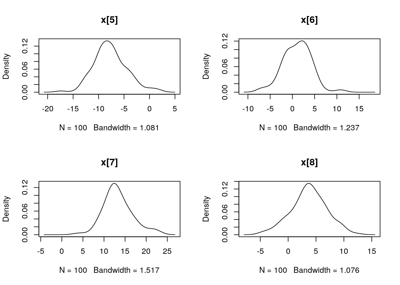
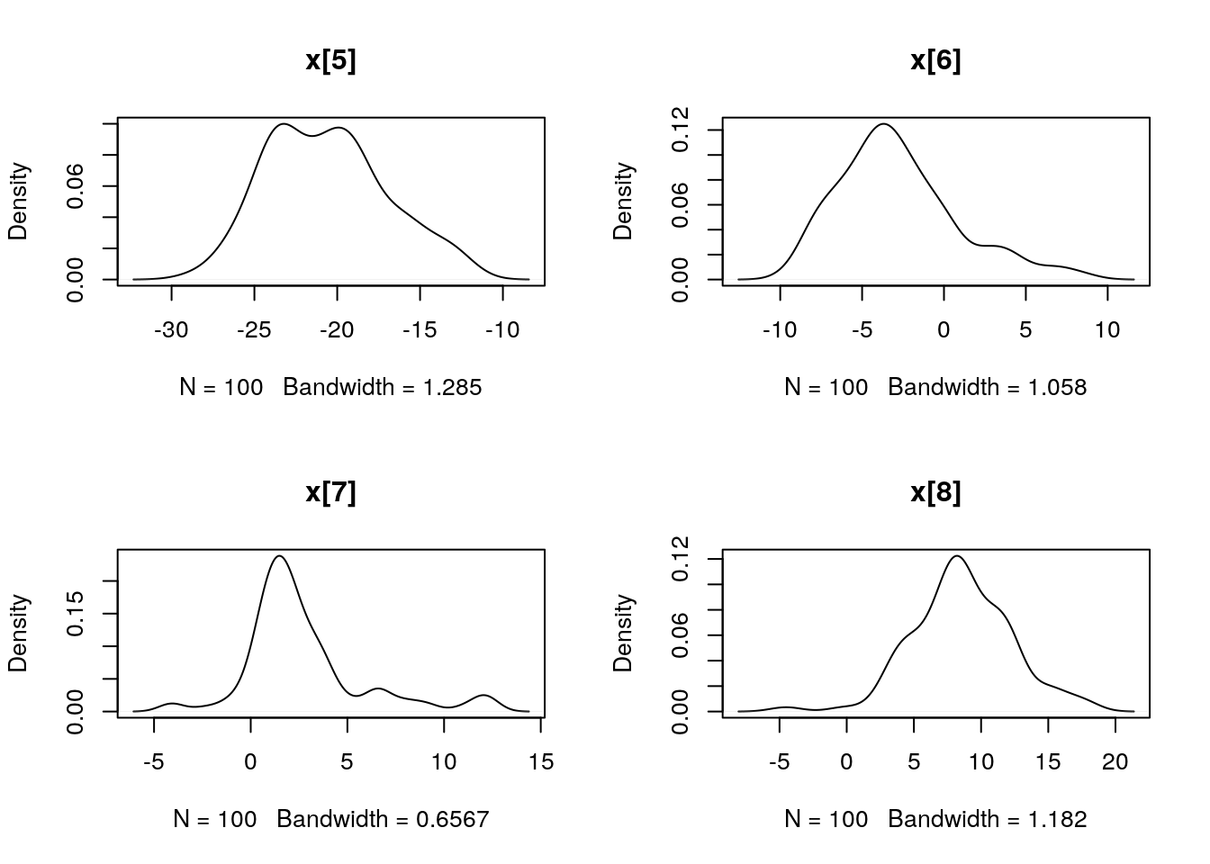
## Marginalizing over: particle(100)dens_smc_x <- biips_density(out_smc$x, bw = 'nrd0', adjust = 1, n = 100)
par(mfrow = c(2, 2))
plot(dens_smc_x)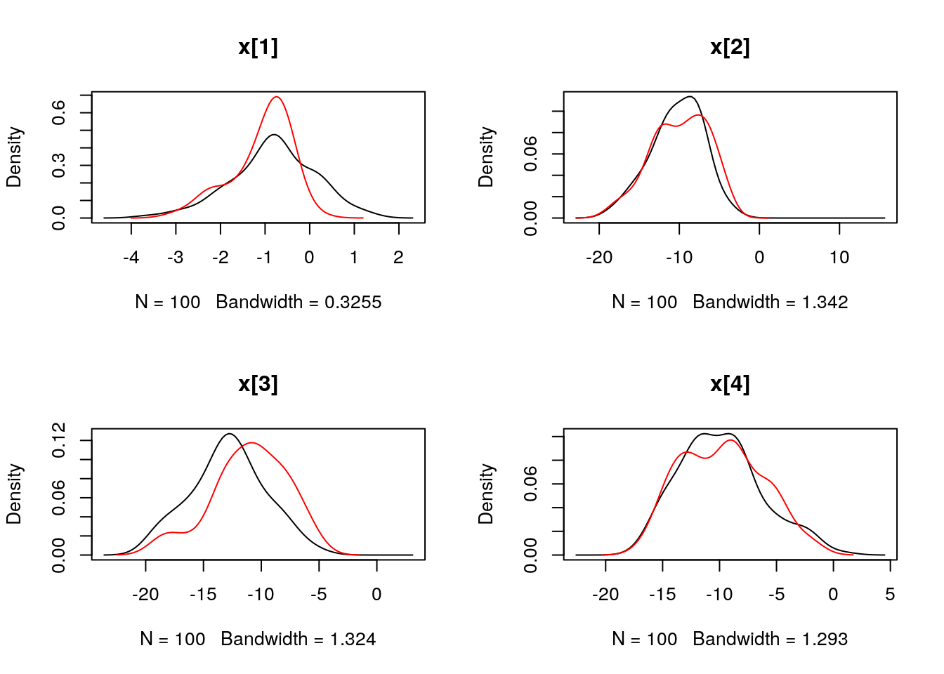
is.smcarray.fsb(out_smc[['c[2:10]']])## [1] TRUEnames(out_smc[['c[2:10]']])## [1] "f" "s"out_smc[['c[2:10]']]## filtering smcarray:
## $mode
## [1] 1 1 2 1 1 1 1 1 1
##
## Marginalizing over: particle(100)
##
## smoothing smcarray:
## $mode
## [1] 1 1 2 2 1 1 1 1 1
##
## Marginalizing over: particle(100)biips_diagnosis(out_smc[['c[2:10]']])## * Diagnosis of variable: c[2:10]
## Filtering: GOOD
## Smoothing: POOR
## The minimum effective sample size is too low: 27.97195
## Estimates may be poor for some variables.
## You should increase the number of particles
## .summ_smc_c <- biips_summary(out_smc[['c[2:10]']])
summ_smc_c## filtering smcarray:
## $mode
## [1] 1 1 2 1 1 1 1 1 1
##
## Marginalizing over: particle(100)
##
## smoothing smcarray:
## $mode
## [1] 1 1 2 2 1 1 1 1 1
##
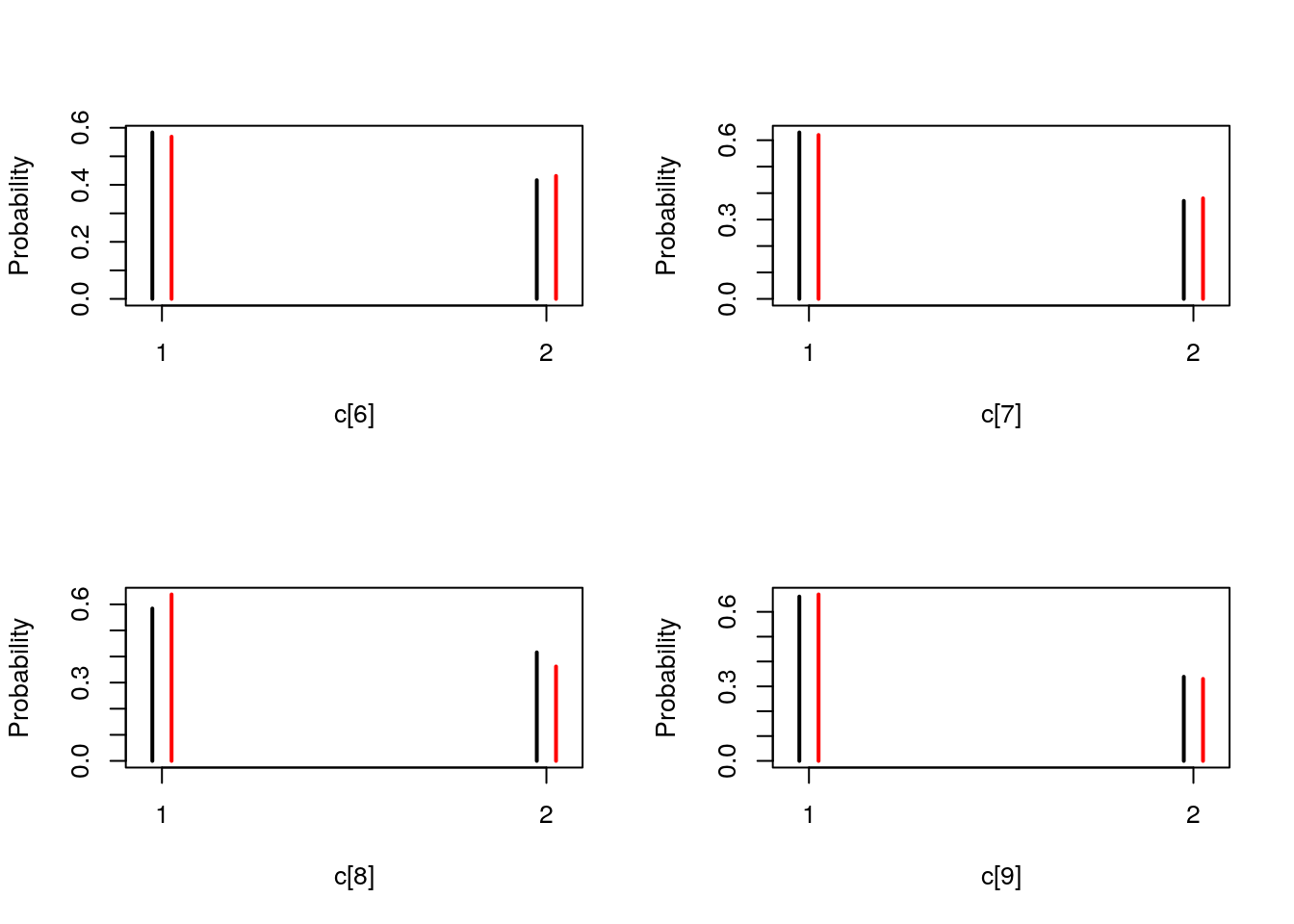
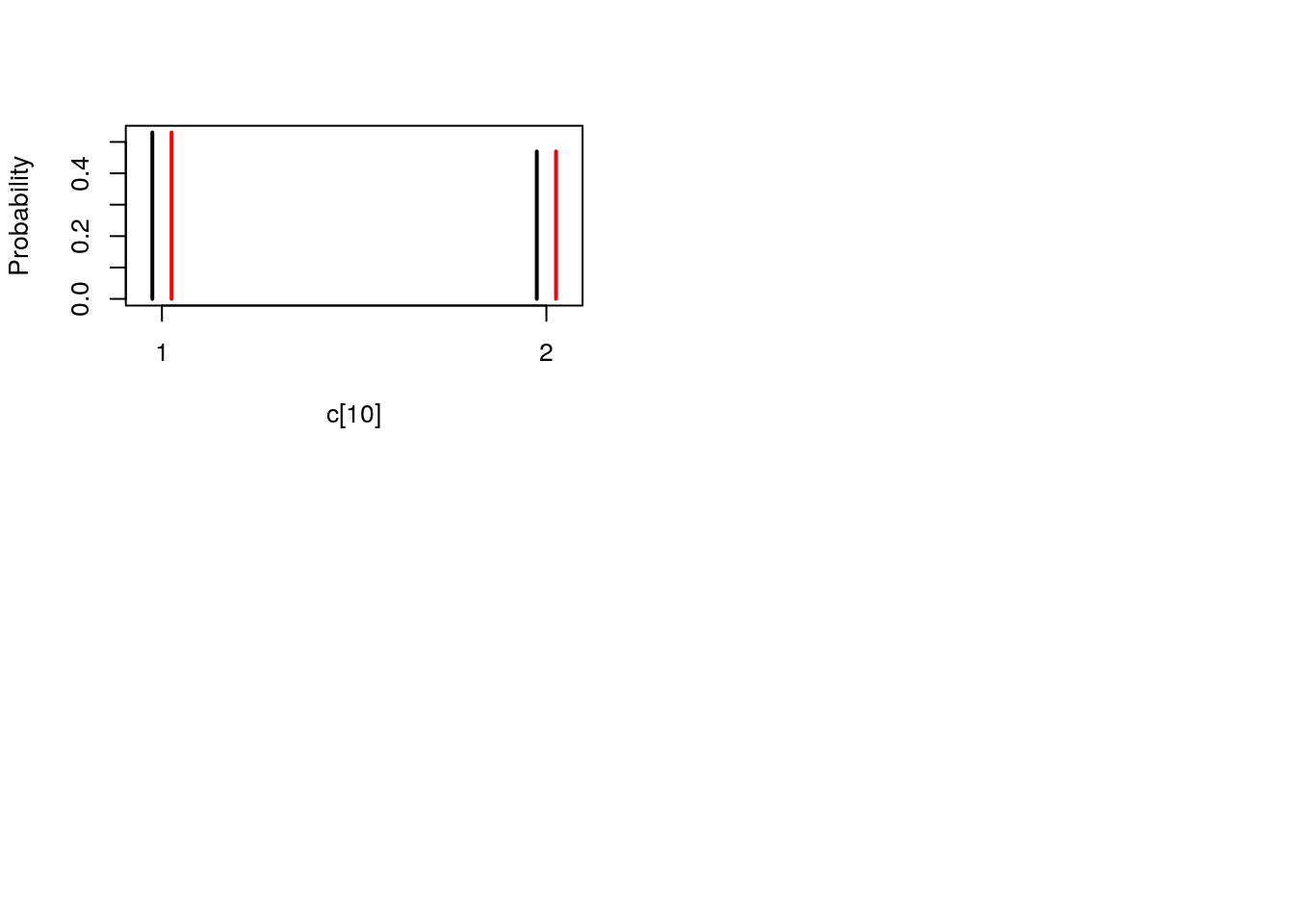
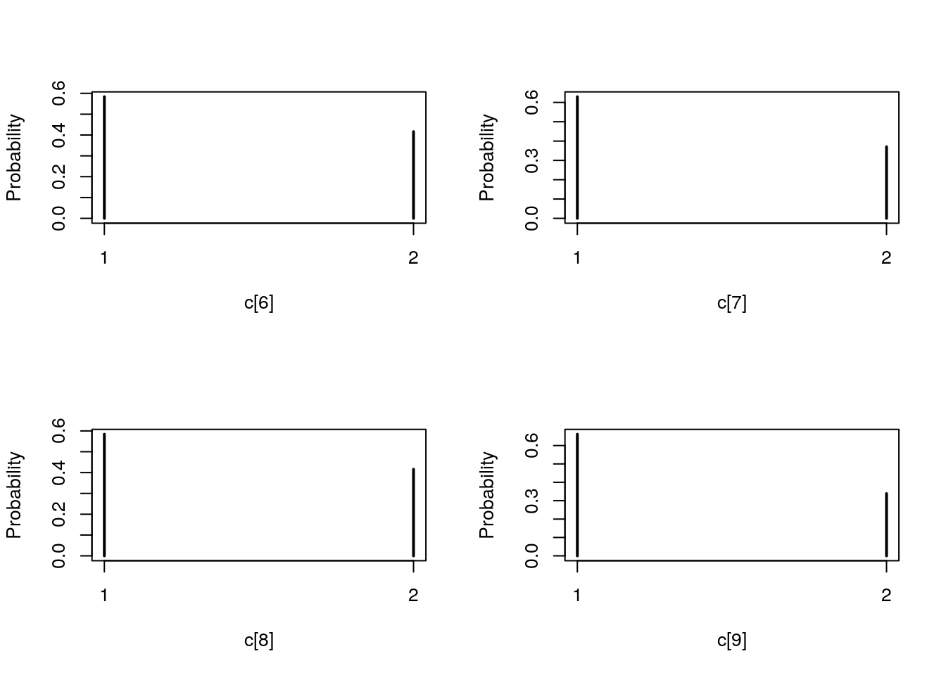
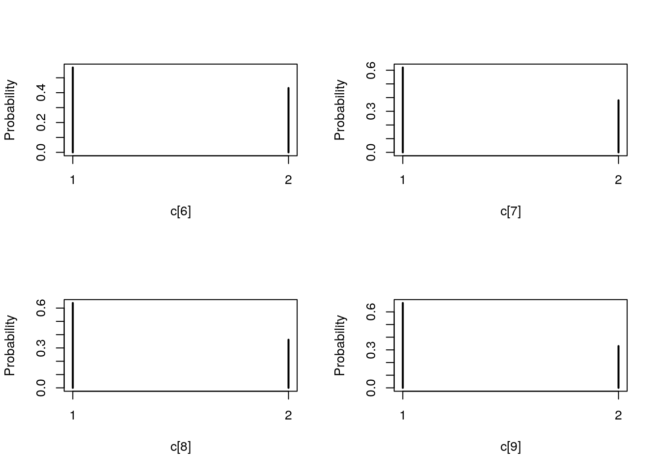
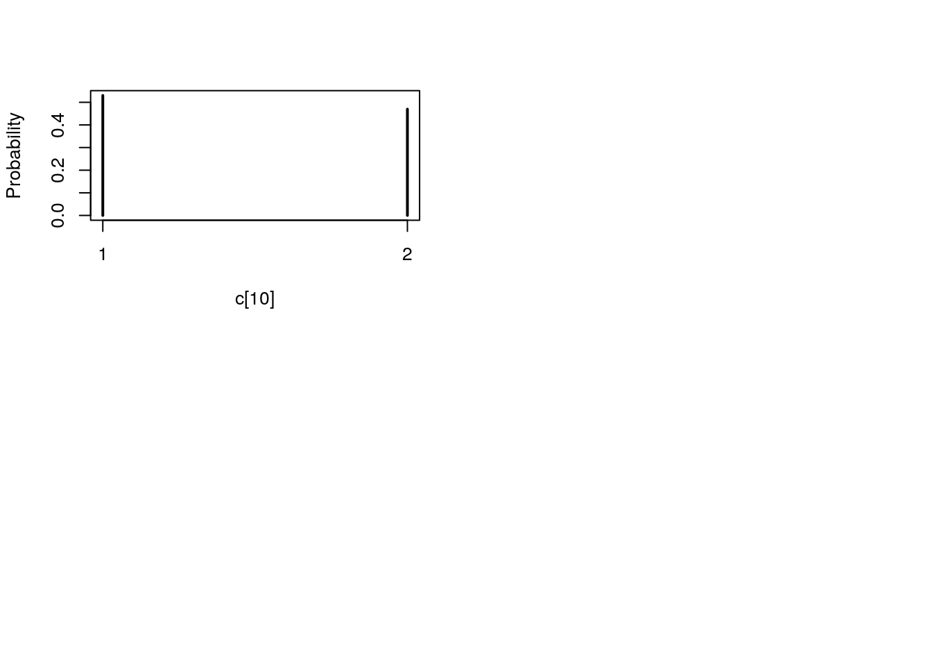
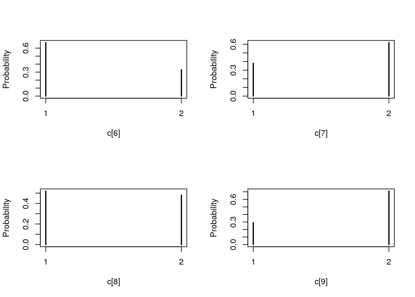
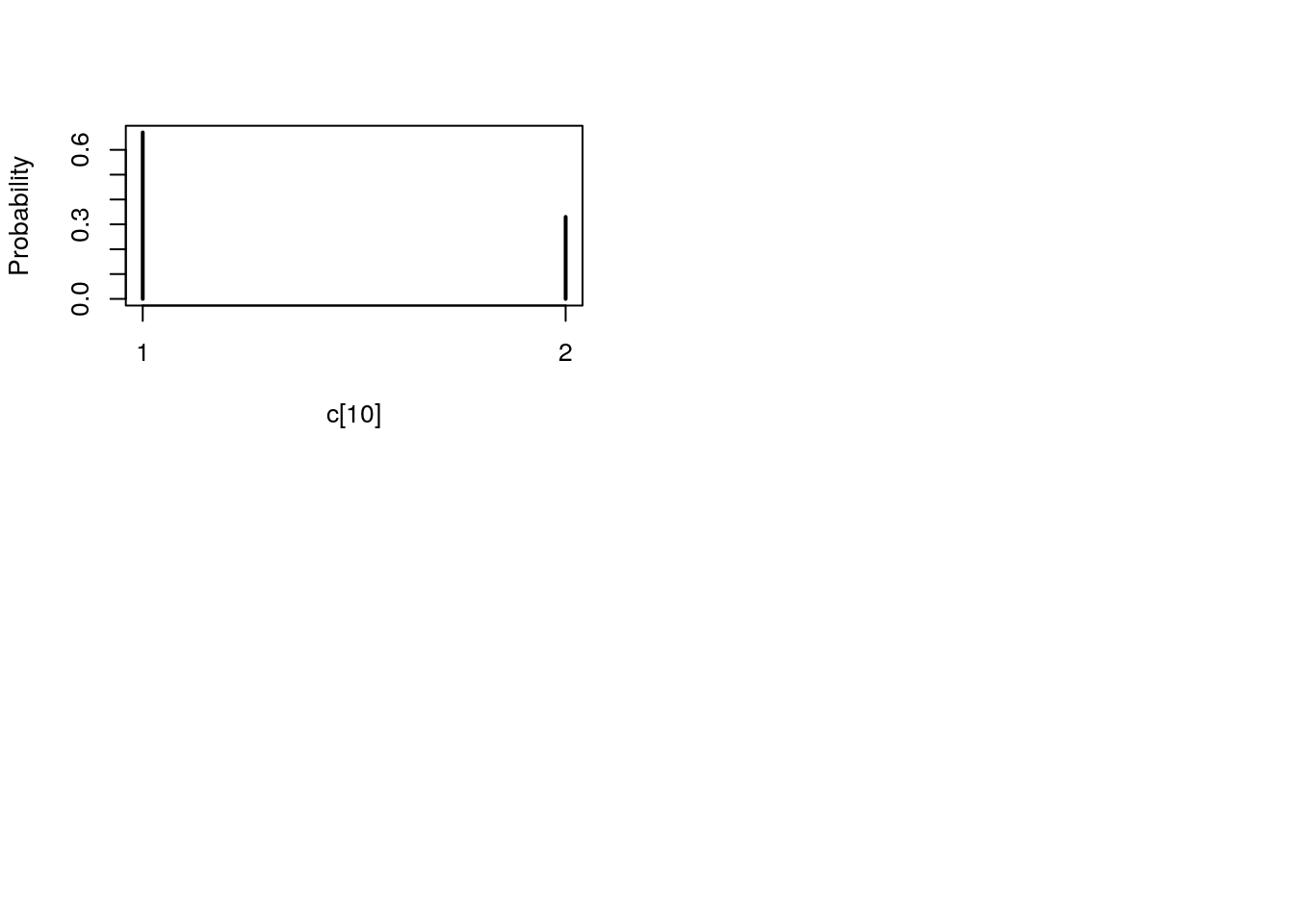
## Marginalizing over: particle(100)table_smc_c <- biips_table(out_smc[['c[2:10]']])
par(mfrow = c(2, 2))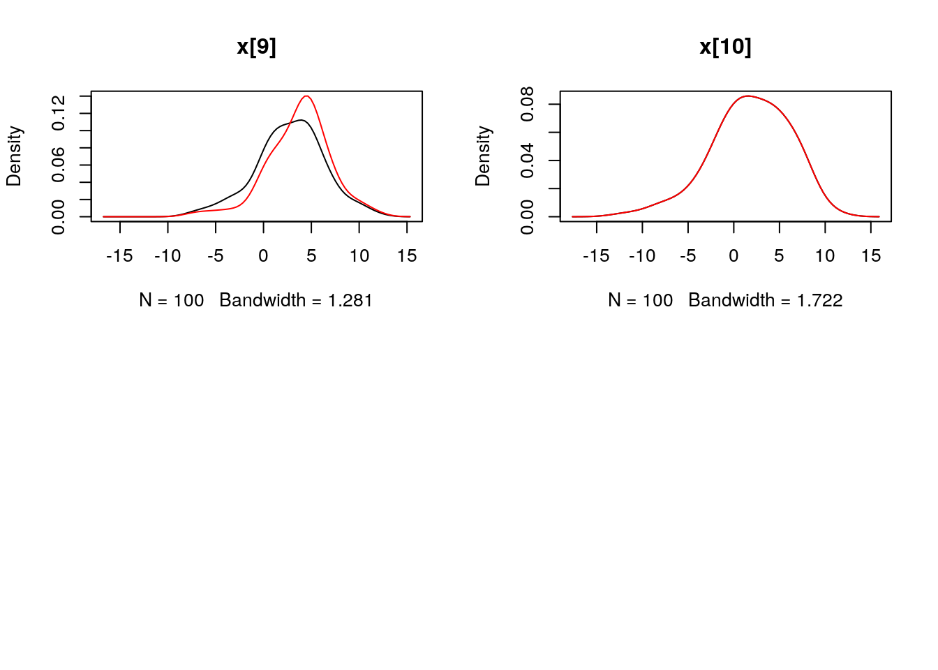
plot(table_smc_c)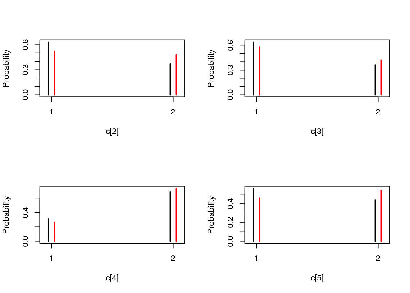
Manipulate smcarray object
is.smcarray(out_smc$x$f)## [1] TRUEnames(out_smc$x$f)## [1] "values" "weights" "ess" "discrete"
## [5] "iterations" "conditionals" "name" "lower"
## [9] "upper" "type"out_smc$x$f## smcarray:
## $mean
## [1] -0.8185253 -10.2517614 -12.8818052 -9.8706867 -7.6815614
## [6] 1.0595768 13.3149162 3.7425798 2.7491513 1.8215615
##
## Marginalizing over: particle(100)out_smc$x$s## smcarray:
## $mean
## [1] -1.075535 -9.946487 -11.013764 -9.784847 -7.637991 2.329093
## [7] 13.109354 4.027466 3.708989 1.821561
##
## Marginalizing over: particle(100)biips_diagnosis(out_smc$x$f)## * Diagnosis of variable: x[1:10]
## Filtering: GOODbiips_diagnosis(out_smc$x$s)## * Diagnosis of variable: x[1:10]
## Smoothing: POOR
## The minimum effective sample size is too low: 27.97195
## Estimates may be poor for some variables.
## You should increase the number of particles
## .biips_summary(out_smc$x$f)## smcarray:
## $mean
## [1] -0.8185253 -10.2517614 -12.8818052 -9.8706867 -7.6815614
## [6] 1.0595768 13.3149162 3.7425798 2.7491513 1.8215615
##
## Marginalizing over: particle(100)biips_summary(out_smc$x$s)## smcarray:
## $mean
## [1] -1.075535 -9.946487 -11.013764 -9.784847 -7.637991 2.329093
## [7] 13.109354 4.027466 3.708989 1.821561
##
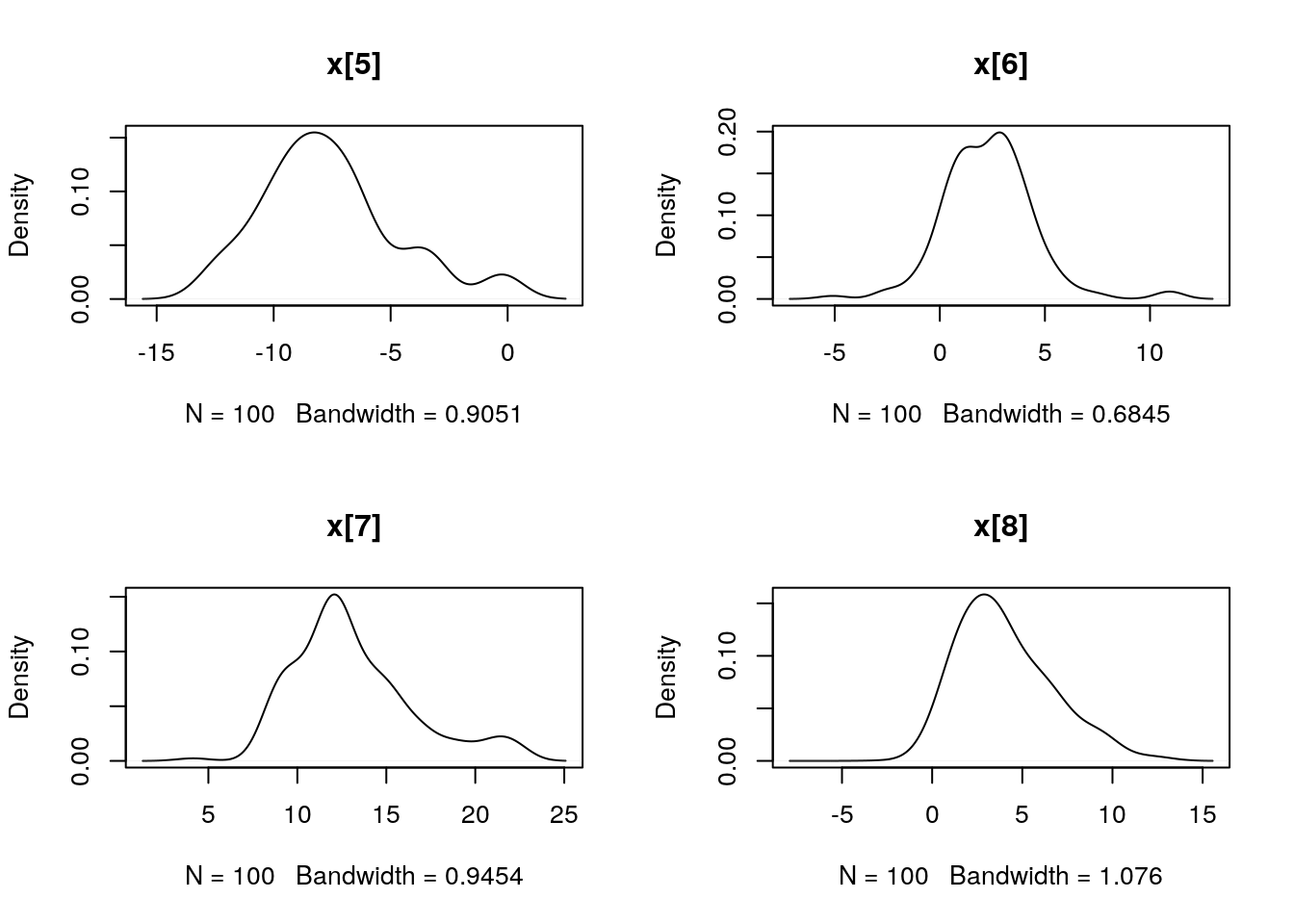
## Marginalizing over: particle(100)par(mfrow = c(2, 2))
plot(biips_density(out_smc$x$f))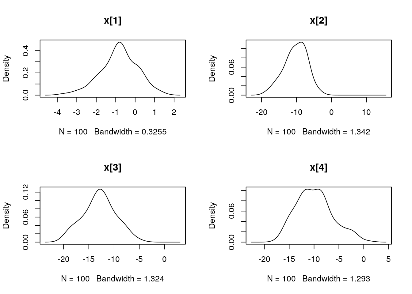
par(mfrow = c(2, 2))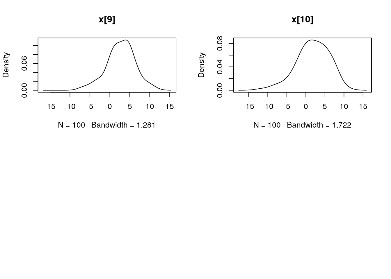
plot(biips_density(out_smc$x$s))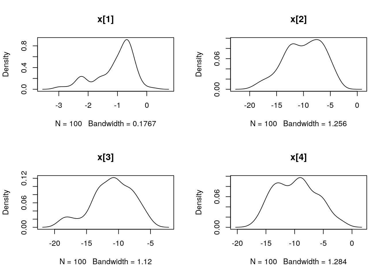
par(mfrow = c(2, 2))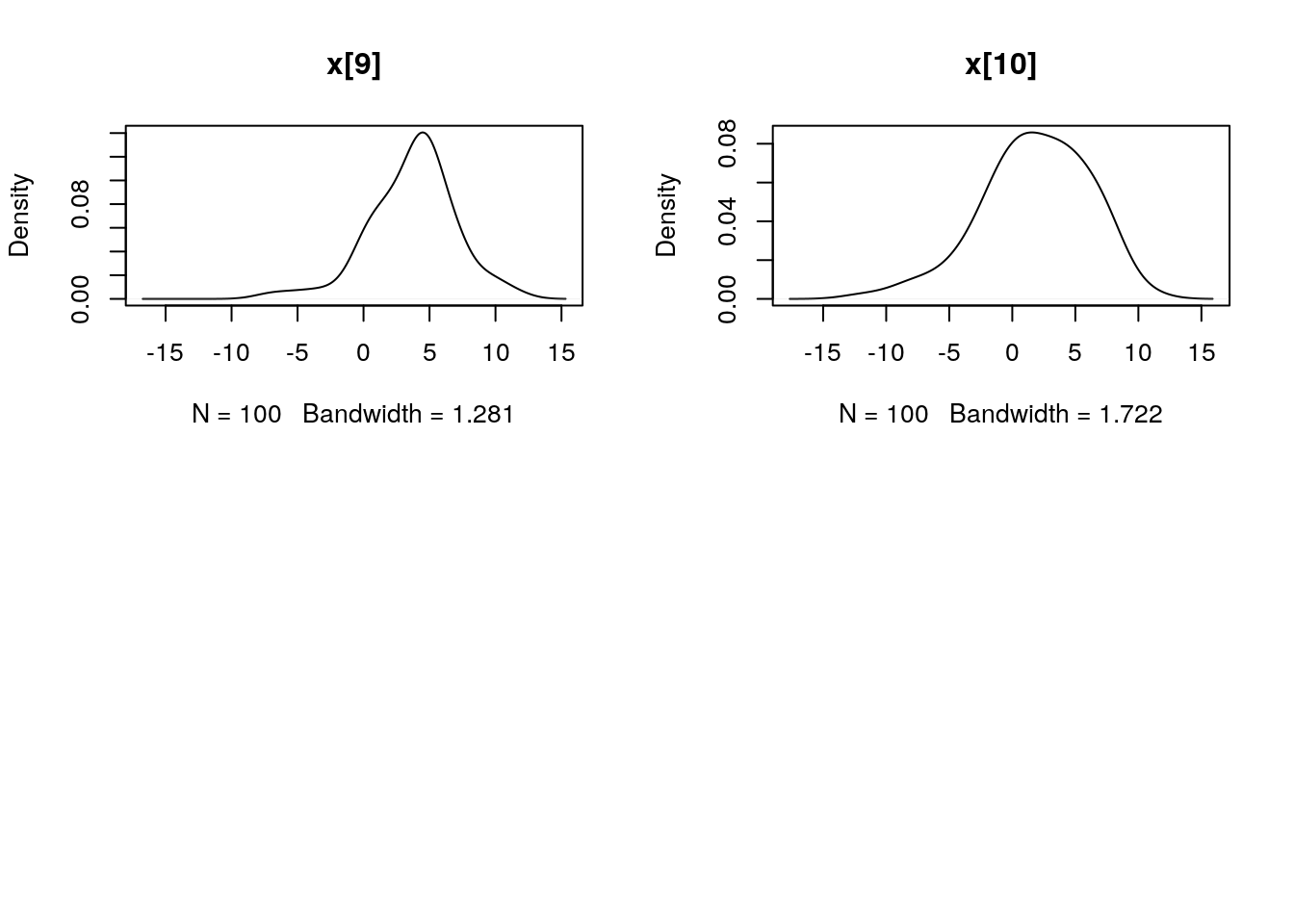
plot(biips_table(out_smc[['c[2:10]']]$f))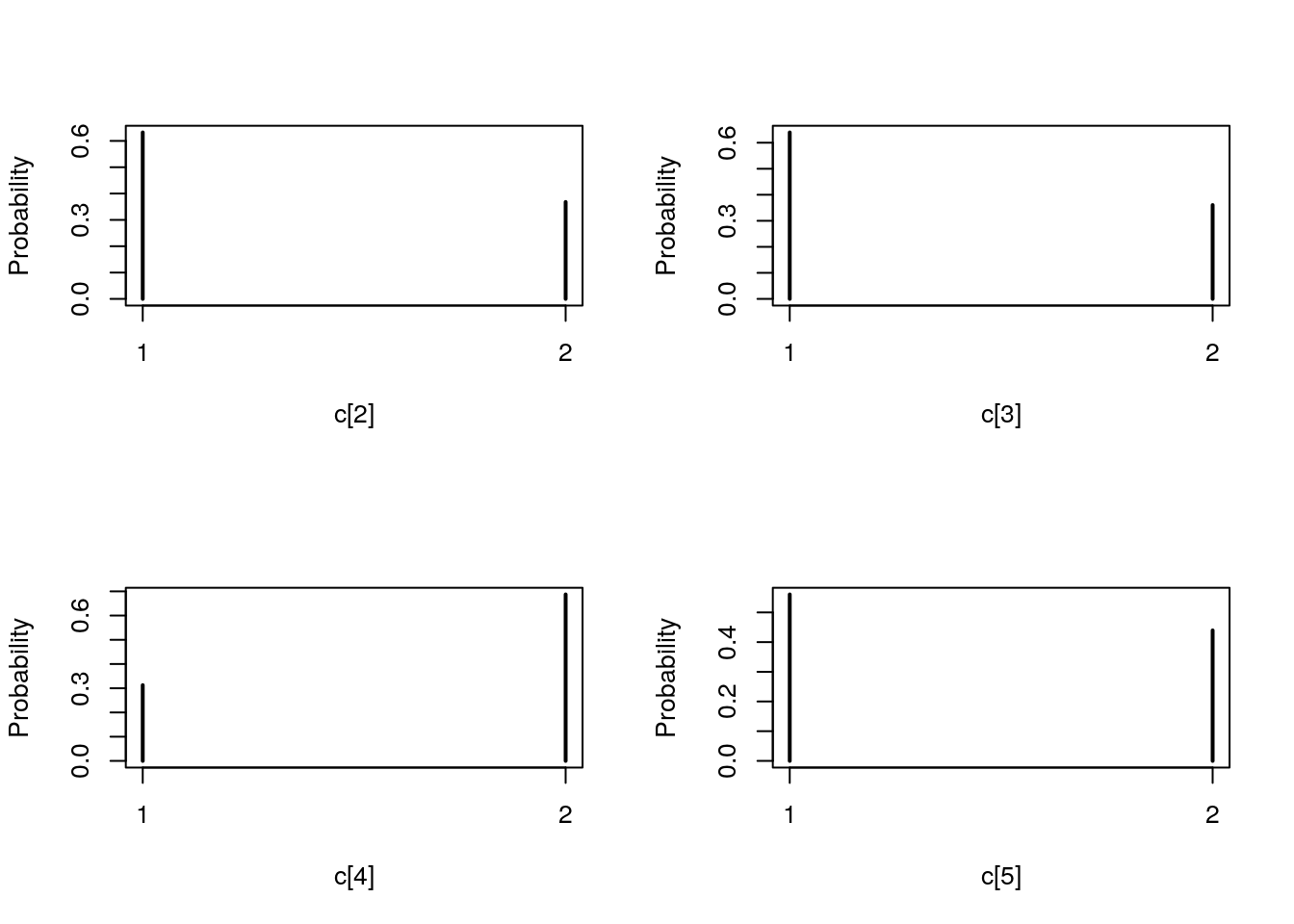
par(mfrow = c(2, 2))
plot(biips_table(out_smc[['c[2:10]']]$s))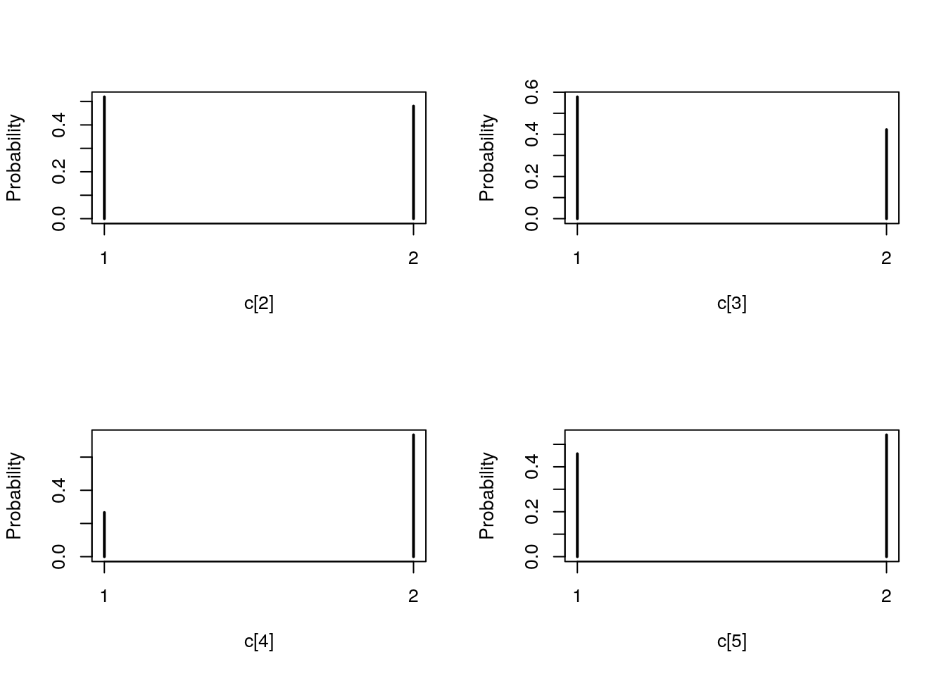
par(mfrow = c(2, 2))
plot(model$data()$x_true, type = 'l', col = 'green', xlab = 't', ylab = 'x[t]')
lines(summ_smc_x$f$mean, col = 'blue')
lines(summ_smc_x$s$mean, col = 'red')
matlines(matrix(unlist(summ_smc_x$f$quant), data$tmax), lty = 2, col = 'blue')
matlines(matrix(unlist(summ_smc_x$s$quant), data$tmax), lty = 2, col = 'red')
legend('topright', leg = c('true', 'SMC filtering estimate', 'SMC smoothing estimate'),
  lty = 1, col = c('green', 'blue', 'red'), bty = 'n')

barplot(.5*(model$data()$c_true==1), col = 'green', border = NA, space = 0, offset=2,
        ylim=c(0,3), xlab='t', ylab='c[t]==1', axes = FALSE)
axis(1, at=1:data$tmax-.5, labels=1:data$tmax)
axis(2, line = 1, at=c(0,3), labels=NA)
text(data$tmax/2, 2.75, 'true')
barplot(.5*c(NA, summ_smc_c$f$mode==1), col = 'blue', border = NA, space = 0,
        offset=1, axes = FALSE, add = TRUE)
text(data$tmax/2, 1.75, 'SMC filtering mode')
barplot(.5*c(NA, summ_smc_c$s$mode==1), col = 'red', border = NA, space = 0,
        axes = FALSE, add = TRUE)
text(data$tmax/2, .75, 'SMC smoothing mode')

t <- 5
plot(dens_smc_x[[t]], col = c('blue','red'), ylab = 'posterior density')
points(model$data()$x_true[t], 0, pch = 17, col = 'green')

plot(table_smc_c[[t-1]], col = c('blue','red'), ylab = 'posterior probability mass')
points(model$data()$c_true[t], 0, pch = 17, col = 'green')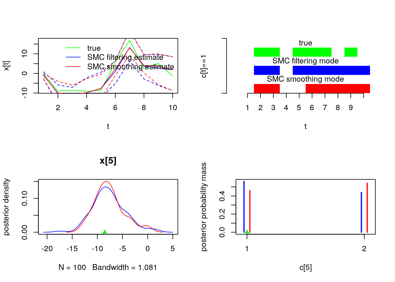
PIMH algorithm
modelfile <- system.file('extdata', 'hmm.bug', package = 'rbiips')
stopifnot(nchar(modelfile) > 0)
cat(readLines(modelfile), sep = '\n')
## var c_true[tmax], x_true[tmax], c[tmax], x[tmax], y[tmax]
##
## data
## {
## x_true[1] ~ dnorm(0, 1/5)
## y[1] ~ dnorm(x_true[1], exp(logtau_true))
## for (t in 2:tmax)
## {
## c_true[t] ~ dcat(p)
## x_true[t] ~ dnorm(0.5*x_true[t-1]+25*x_true[t-1]/(1+x_true[t-1]^2)+8*cos(1.2*(t-1)), ifelse(c_true[t]==1, 1/10, 1/100))
## y[t] ~ dnorm(x_true[t]/4, exp(logtau_true))
## }
## }
##
## model
## {
## logtau ~ dunif(-3, 3)
## x[1] ~ dnorm(0, 1/5)
## y[1] ~ dnorm(x[1], exp(logtau))
## for (t in 2:tmax)
## {
## c[t] ~ dcat(p)
## x[t] ~ dnorm(0.5*x[t-1]+25*x[t-1]/(1+x[t-1]^2)+8*cos(1.2*(t-1)), ifelse(c[t]==1, 1/10, 1/100))
## y[t] ~ dnorm(x[t]/4, exp(logtau))
## }
## }data <- list(tmax = 10, p = c(.5, .5), logtau_true = log(1), logtau = log(1))
model <- biips_model(modelfile, data)## * Parsing model in: /home/adrien/R/x86_64-pc-linux-gnu-library/3.4/rbiips/extdata/hmm.bug
## * Compiling data graph
## Declaring variables
## Resolving undeclared variables
## Allocating nodes
## Graph size: 169
## Sampling data
## Reading data back into data table
## * Compiling model graph
## Declaring variables
## Resolving undeclared variables
## Allocating nodes
## Graph size: 180n_part <- 50
obj_pimh <- biips_pimh_init(model, c('x', 'c[2:10]')) # Initialize## * Initializing PIMHis.pimh(obj_pimh)## [1] TRUEout_pimh_burn <- biips_pimh_update(obj_pimh, 100, n_part) # Burn-in## * Updating PIMH with 50 particles
## |--------------------------------------------------| 100%
## |**************************************************| 100 iterations in 0.33 sout_pimh <- biips_pimh_samples(obj_pimh, 100, n_part) # Samples## * Generating PIMH samples with 50 particles
## |--------------------------------------------------| 100%
## |**************************************************| 100 iterations in 0.29 sManipulate mcmcarray.list object
is.mcmcarray.list(out_pimh)## [1] TRUEnames(out_pimh)## [1] "log_marg_like" "x" "c[2:10]"out_pimh## x mcmcarray:
## $mean
## [1] -1.744318 -6.360808 -10.321973 -17.901901 -20.619587 -2.810113
## [7] 2.725313 8.596764 -7.292871 -9.084865
##
## Marginalizing over: iteration(100)
##
## c[2:10] mcmcarray:
## $mode
## [1] 1 1 1 2 1 2 1 2 1
##
## Marginalizing over: iteration(100)biips_summary(out_pimh)## x mcmcarray:
## $mean
## [1] -1.744318 -6.360808 -10.321973 -17.901901 -20.619587 -2.810113
## [7] 2.725313 8.596764 -7.292871 -9.084865
##
## Marginalizing over: iteration(100)
##
## c[2:10] mcmcarray:
## $mode
## [1] 1 1 1 2 1 2 1 2 1
##
## Marginalizing over: iteration(100)Manipulate mcmcarray object
is.mcmcarray(out_pimh$x)## [1] TRUEout_pimh$x## mcmcarray:
## $mean
## [1] -1.744318 -6.360808 -10.321973 -17.901901 -20.619587 -2.810113
## [7] 2.725313 8.596764 -7.292871 -9.084865
##
## Marginalizing over: iteration(100)summ_pimh_x <- biips_summary(out_pimh$x, order = 2, probs = c(0.025, 0.975))
summ_pimh_x## mcmcarray:
## $mean
## [1] -1.744318 -6.360808 -10.321973 -17.901901 -20.619587 -2.810113
## [7] 2.725313 8.596764 -7.292871 -9.084865
##
## $var
## [1] 0.7759045 7.5914789 11.4434933 10.9032501 12.8568713 13.4999635
## [7] 9.7265090 13.6051737 12.4830571 8.3317342
##
## $probs
## [1] 0.025 0.975
##
## $quant
## $quant$`0.025`
## [1] -3.181049 -10.646213 -17.866211 -26.847726 -26.370300 -8.137910
## [7] -1.813076 2.640606 -14.564996 -15.282659
##
## $quant$`0.975`
## [1] -0.2613017 -0.2260500 -3.9108981 -13.7375080 -13.1618345
## [6] 6.1863795 12.0359348 16.0097494 -2.0332459 -4.2237906
##
##
## Marginalizing over: iteration(100)dens_pimh_x <- biips_density(out_pimh$x)
par(mfrow = c(2, 2))
plot(dens_pimh_x)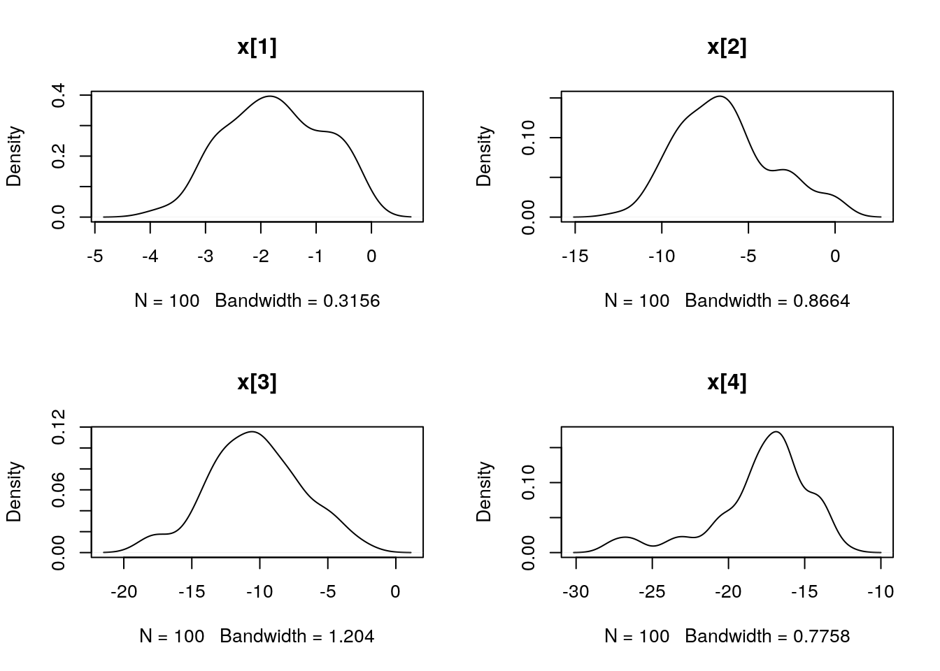
par(mfrow = c(2, 2))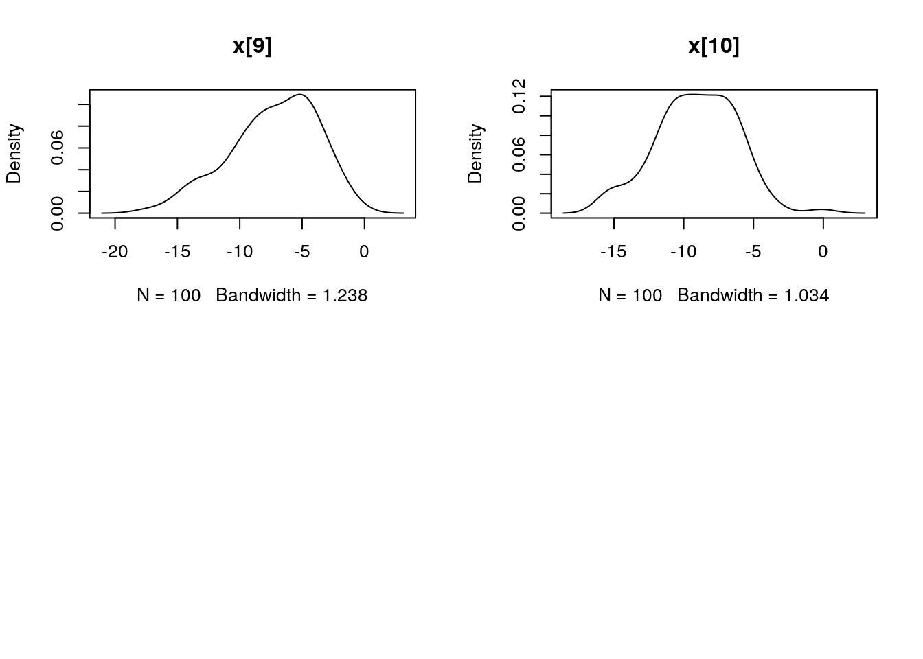
biips_hist(out_pimh$x)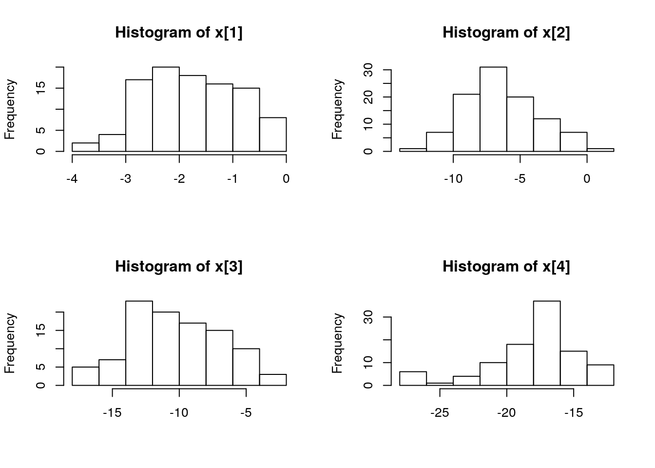

is.mcmcarray(out_pimh[['c[2:10]']])## [1] TRUEout_pimh[['c[2:10]']]## mcmcarray:
## $mode
## [1] 1 1 1 2 1 2 1 2 1
##
## Marginalizing over: iteration(100)summ_pimh_c <- biips_summary(out_pimh[['c[2:10]']])
summ_pimh_c## mcmcarray:
## $mode
## [1] 1 1 1 2 1 2 1 2 1
##
## Marginalizing over: iteration(100)table_pimh_c <- biips_table(out_pimh[['c[2:10]']])
par(mfrow = c(2, 2))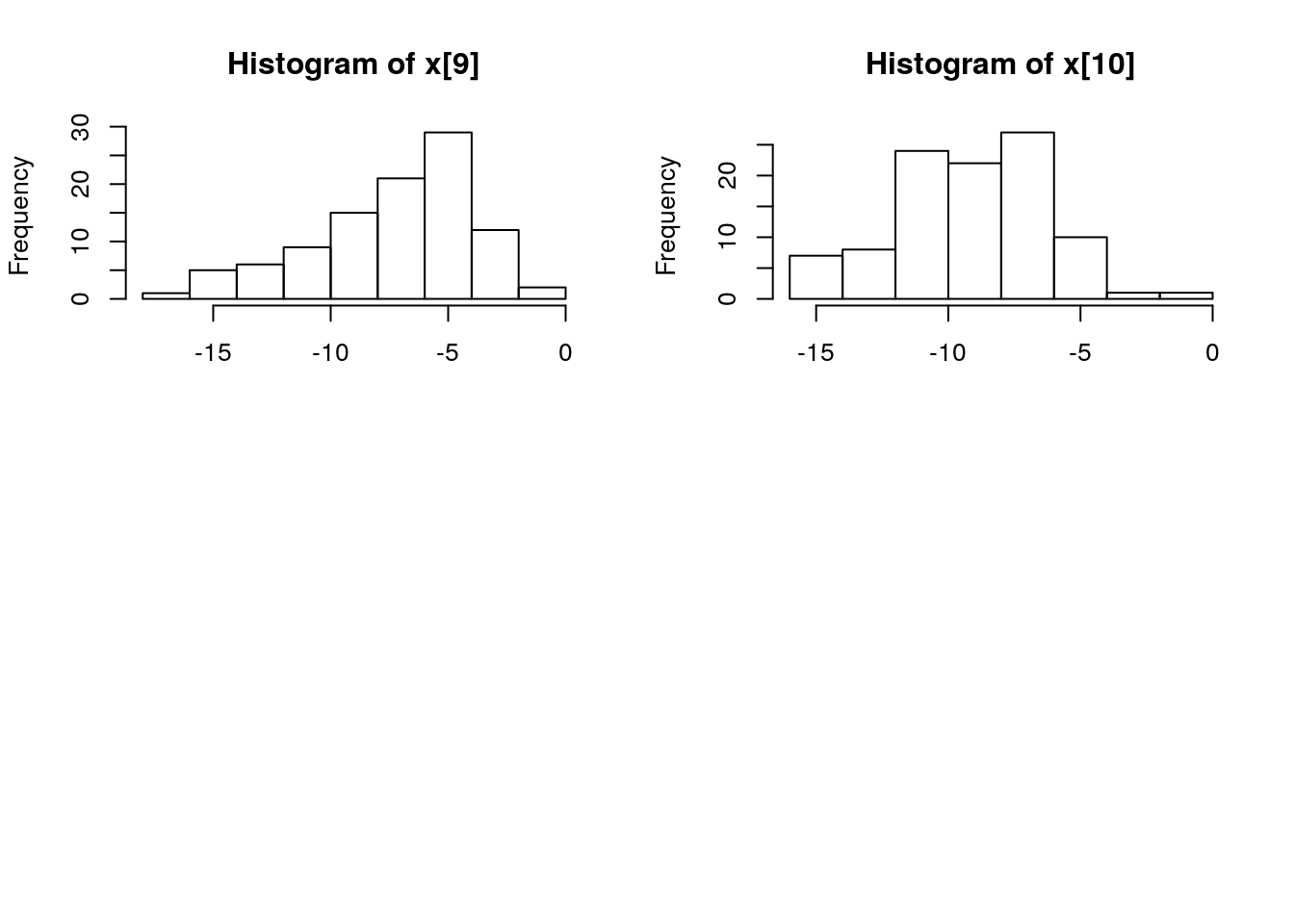
plot(table_pimh_c)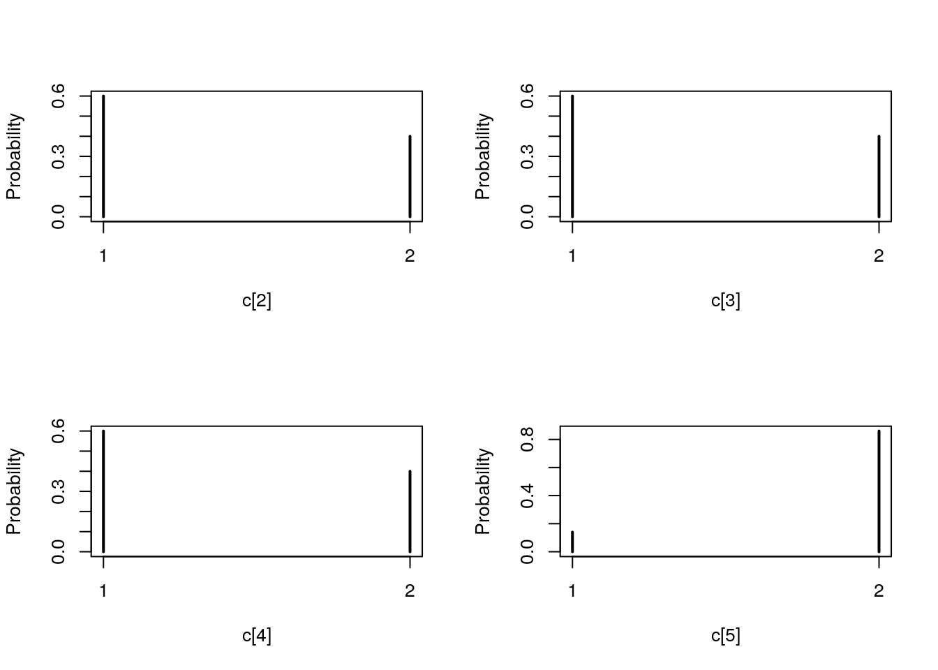
par(mfrow = c(2, 1))
plot(c(out_pimh_burn$log_marg_like, out_pimh$log_marg_like), type = 'l', col = 'blue',
  xlab = 'PIMH iteration', ylab = 'log p(y)')

t <- 5
plot(out_pimh$x[t, ], type = 'l', col = 'blue', xlab = 'PIMH iteration',
     ylab = paste0('x[',t,']'))
points(0, model$data()$x_true[t], pch = 17, col = 'green')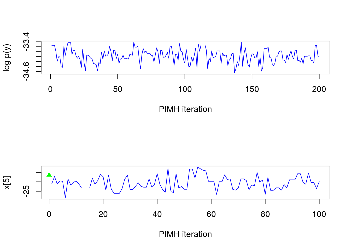
par(mfrow = c(2, 2))
plot(model$data()$x_true, type = 'l', col = 'green', xlab = 't', ylab = 'x[t]')
lines(summ_pimh_x$mean, col = 'blue')
matlines(matrix(unlist(summ_pimh_x$quant), data$tmax), lty = 2, col = 'blue')
legend('topright', leg = c('true', 'PIMH estimate'), lty = c(2, 1), col = c('green',
  'blue'), bty = 'n')

barplot(.5*(model$data()$c_true==1), col = 'green', border = NA, space = 0, offset = 1,
        ylim=c(0,2), xlab='t', ylab='c[t]==1', axes = FALSE)
axis(1, at=1:data$tmax-.5, labels=1:data$tmax)
axis(2, line = 1, at=c(0,2), labels=NA)
text(data$tmax/2, 1.75, 'true')
barplot(.5*c(NA, summ_pimh_c$mode==1), col = 'blue', border = NA, space = 0, axes = FALSE, add = TRUE)
text(data$tmax/2, .75, 'PIMH mode')

plot(dens_pimh_x[[t]], col='blue', main = , ylab = 'posterior density')
points(model$data()$x_true[t], 0, pch = 17, col = 'green')

plot(table_pimh_c[[t-1]], col='blue', ylab = 'posterior probability mass')
points(model$data()$c_true[t], 0, pch = 17, col = 'green')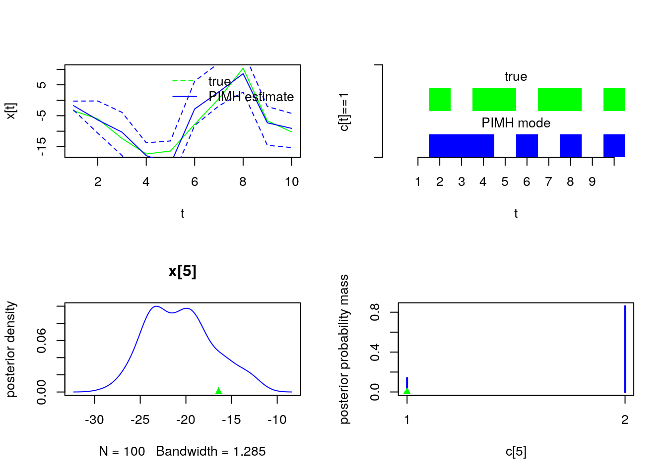
SMC sensitivity analysis
modelfile <- system.file('extdata', 'hmm.bug', package = 'rbiips')
stopifnot(nchar(modelfile) > 0)
cat(readLines(modelfile), sep = '\n')
## var c_true[tmax], x_true[tmax], c[tmax], x[tmax], y[tmax]
##
## data
## {
## x_true[1] ~ dnorm(0, 1/5)
## y[1] ~ dnorm(x_true[1], exp(logtau_true))
## for (t in 2:tmax)
## {
## c_true[t] ~ dcat(p)
## x_true[t] ~ dnorm(0.5*x_true[t-1]+25*x_true[t-1]/(1+x_true[t-1]^2)+8*cos(1.2*(t-1)), ifelse(c_true[t]==1, 1/10, 1/100))
## y[t] ~ dnorm(x_true[t]/4, exp(logtau_true))
## }
## }
##
## model
## {
## logtau ~ dunif(-3, 3)
## x[1] ~ dnorm(0, 1/5)
## y[1] ~ dnorm(x[1], exp(logtau))
## for (t in 2:tmax)
## {
## c[t] ~ dcat(p)
## x[t] ~ dnorm(0.5*x[t-1]+25*x[t-1]/(1+x[t-1]^2)+8*cos(1.2*(t-1)), ifelse(c[t]==1, 1/10, 1/100))
## y[t] ~ dnorm(x[t]/4, exp(logtau))
## }
## }data <- list(tmax = 10, p = c(.5, .5), logtau_true = log(1), logtau = log(1))
model <- biips_model(modelfile, data)## * Parsing model in: /home/adrien/R/x86_64-pc-linux-gnu-library/3.4/rbiips/extdata/hmm.bug
## * Compiling data graph
## Declaring variables
## Resolving undeclared variables
## Allocating nodes
## Graph size: 169
## Sampling data
## Reading data back into data table
## * Compiling model graph
## Declaring variables
## Resolving undeclared variables
## Allocating nodes
## Graph size: 180n_part <- 50
logtau_val <- -10:10
out_sens <- biips_smc_sensitivity(model, list(logtau = logtau_val), n_part)## * Analyzing sensitivity with 50 particles
## |--------------------------------------------------| 100%
## |**************************************************| 21 iterations in 0.05 spar(mfrow = c(2, 1))
plot(logtau_val, out_sens$log_marg_like, type = 'l', col = 'blue',
xlab = 'logtau', ylab = 'log p(y | logtau) ', main = 'SMC sensitivity')
points(data$logtau, min(out_sens$log_marg_like), pch = 17, col = 'green')
plot(logtau_val, out_sens$log_marg_like_pen, type = 'l', col = 'blue',
xlab = 'logtau', ylab = 'log p(y, logtau)')
plml <- out_sens$log_marg_like_pen
ymin <- min(plml[is.finite(plml)])
points(data$logtau, ymin, pch = 17, col = 'green')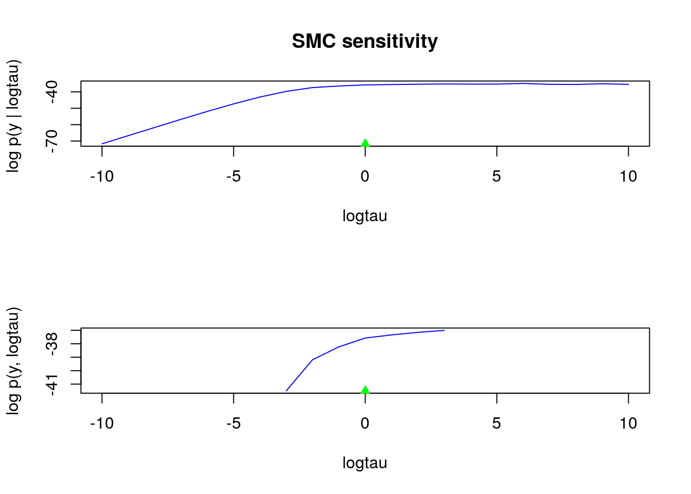
PMMH algorithm
modelfile <- system.file('extdata', 'hmm.bug', package = 'rbiips')
stopifnot(nchar(modelfile) > 0)
cat(readLines(modelfile), sep = '\n')
## var c_true[tmax], x_true[tmax], c[tmax], x[tmax], y[tmax]
##
## data
## {
## x_true[1] ~ dnorm(0, 1/5)
## y[1] ~ dnorm(x_true[1], exp(logtau_true))
## for (t in 2:tmax)
## {
## c_true[t] ~ dcat(p)
## x_true[t] ~ dnorm(0.5*x_true[t-1]+25*x_true[t-1]/(1+x_true[t-1]^2)+8*cos(1.2*(t-1)), ifelse(c_true[t]==1, 1/10, 1/100))
## y[t] ~ dnorm(x_true[t]/4, exp(logtau_true))
## }
## }
##
## model
## {
## logtau ~ dunif(-3, 3)
## x[1] ~ dnorm(0, 1/5)
## y[1] ~ dnorm(x[1], exp(logtau))
## for (t in 2:tmax)
## {
## c[t] ~ dcat(p)
## x[t] ~ dnorm(0.5*x[t-1]+25*x[t-1]/(1+x[t-1]^2)+8*cos(1.2*(t-1)), ifelse(c[t]==1, 1/10, 1/100))
## y[t] ~ dnorm(x[t]/4, exp(logtau))
## }
## }data <- list(tmax = 10, p = c(.5, .5), logtau_true = log(1))
model <- biips_model(modelfile, data)## * Parsing model in: /home/adrien/R/x86_64-pc-linux-gnu-library/3.4/rbiips/extdata/hmm.bug
## * Compiling data graph
## Declaring variables
## Resolving undeclared variables
## Allocating nodes
## Graph size: 168
## Sampling data
## Reading data back into data table
## * Compiling model graph
## Declaring variables
## Resolving undeclared variables
## Allocating nodes
## Graph size: 180n_part <- 50
n_burn <- 50
n_iter <- 50
obj_pmmh <- biips_pmmh_init(model, 'logtau', latent_names = c('x', 'c[2:10]'),
inits = list(logtau = -2)) # Initialize## * Initializing PMMHis.pmmh(obj_pmmh)## [1] TRUEout_pmmh_burn <- biips_pmmh_update(obj_pmmh, n_burn, n_part) # Burn-in## * Adapting PMMH with 50 particles
## |--------------------------------------------------| 100%
## |++++++++++++++++++++++++++++++++++++++++++++++++++| 50 iterations in 0.27 sout_pmmh <- biips_pmmh_samples(obj_pmmh, n_iter, n_part, thin = 1) # Samples## * Generating 50 PMMH samples with 50 particles
## |--------------------------------------------------| 100%
## |**************************************************| 50 iterations in 0.18 sManipulate mcmcarray.list object
is.mcmcarray.list(out_pmmh)## [1] TRUEnames(out_pmmh)## [1] "log_marg_like_pen" "logtau" "x"
## [4] "c[2:10]"out_pmmh## logtau mcmcarray:
## $mean
## [1] 1.367072
##
## Marginalizing over: iteration(50)
##
## x mcmcarray:
## $mean
## [1] 0.01569417 6.10443187 1.19944887 27.21569371 13.54589956
## [6] 23.39552012 10.52836336 5.78124480 18.62547890 -3.32506938
##
## Marginalizing over: iteration(50)
##
## c[2:10] mcmcarray:
## $mode
## [1] 1 1 2 1 2 1 1 2 2
##
## Marginalizing over: iteration(50)biips_summary(out_pmmh)## logtau mcmcarray:
## $mean
## [1] 1.367072
##
## Marginalizing over: iteration(50)
##
## x mcmcarray:
## $mean
## [1] 0.01569417 6.10443187 1.19944887 27.21569371 13.54589956
## [6] 23.39552012 10.52836336 5.78124480 18.62547890 -3.32506938
##
## Marginalizing over: iteration(50)
##
## c[2:10] mcmcarray:
## $mode
## [1] 1 1 2 1 2 1 1 2 2
##
## Marginalizing over: iteration(50)Manipulate mcmcarray object
is.mcmcarray(out_pmmh$logtau)## [1] TRUEout_pmmh$logtau## mcmcarray:
## $mean
## [1] 1.367072
##
## Marginalizing over: iteration(50)summ_pmmh_lt <- biips_summary(out_pmmh$logtau, order = 2, probs = c(0.025, 0.975))
dens_pmmh_lt <- biips_density(out_pmmh$logtau)
par(mfrow = c(2, 1))
plot(dens_pmmh_lt)
biips_hist(out_pmmh$logtau)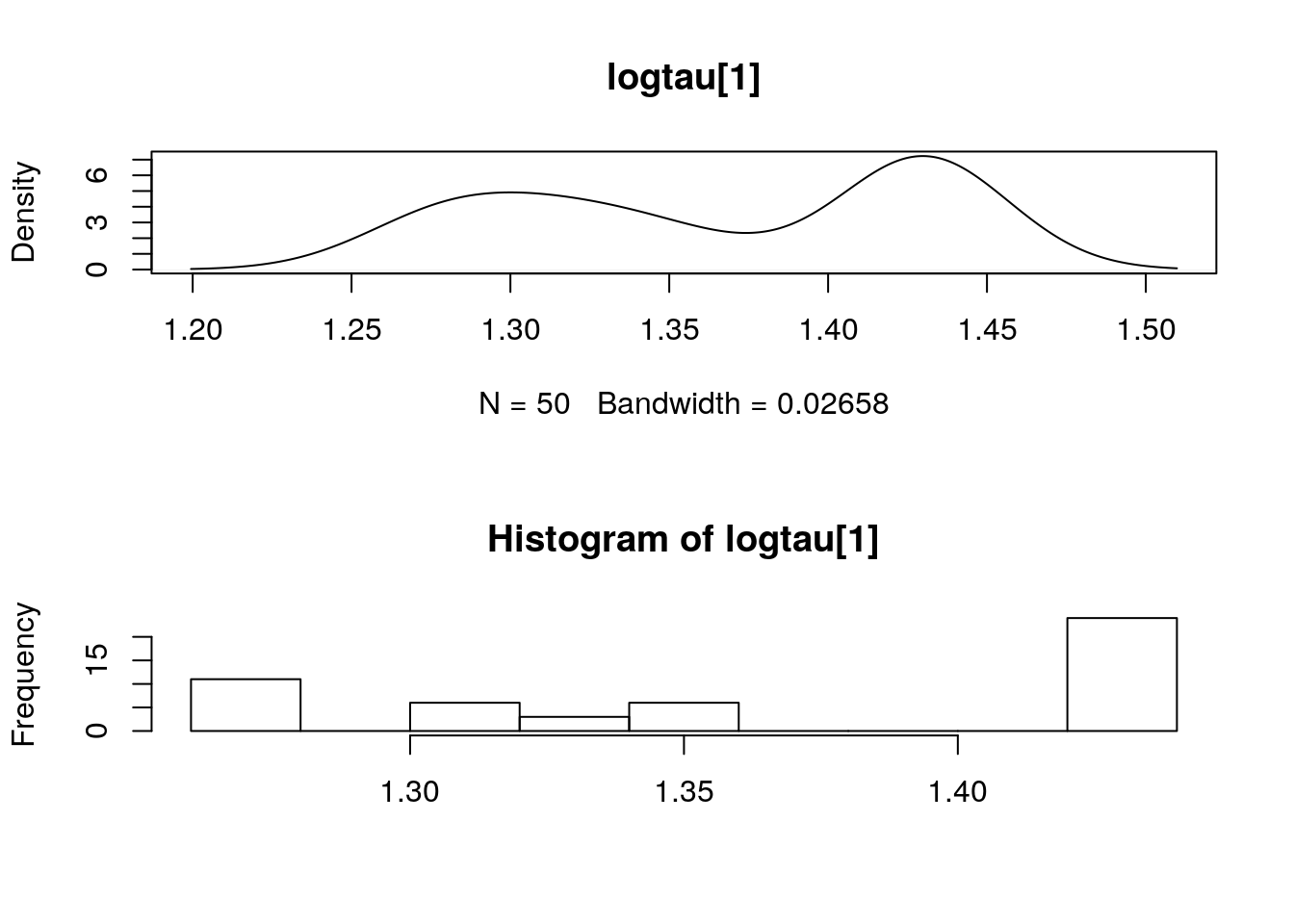
is.mcmcarray(out_pmmh$x)## [1] TRUEout_pmmh$x## mcmcarray:
## $mean
## [1] 0.01569417 6.10443187 1.19944887 27.21569371 13.54589956
## [6] 23.39552012 10.52836336 5.78124480 18.62547890 -3.32506938
##
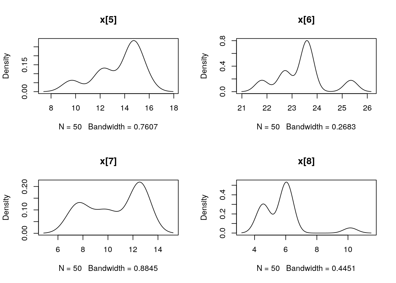
## Marginalizing over: iteration(50)summ_pmmh_x <- biips_summary(out_pmmh$x, order = 2, probs = c(0.025, 0.975))
dens_pmmh_x <- biips_density(out_pmmh$x)
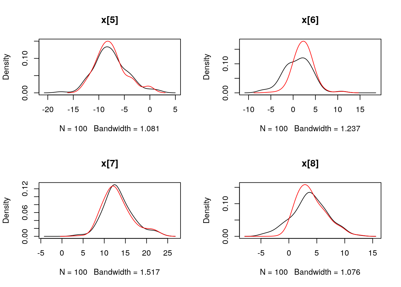
par(mfrow = c(2, 2))
plot(dens_pmmh_x)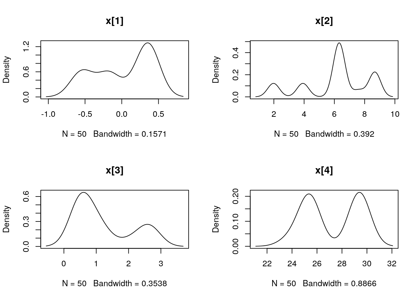
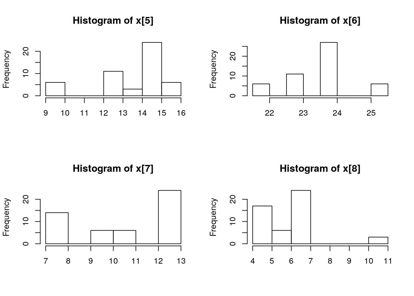
par(mfrow = c(2, 2))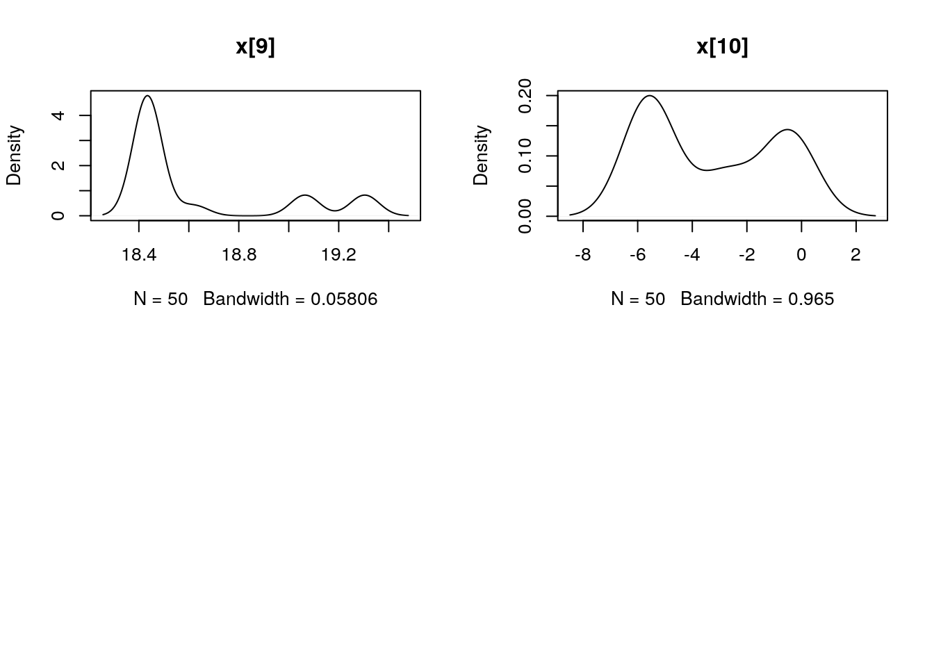
biips_hist(out_pmmh$x)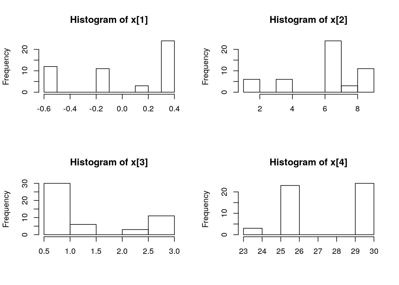
is.mcmcarray(out_pmmh[['c[2:10]']])## [1] TRUEout_pmmh[['c[2:10]']]## mcmcarray:
## $mode
## [1] 1 1 2 1 2 1 1 2 2
##
## Marginalizing over: iteration(50)summ_pmmh_c <- biips_summary(out_pmmh[['c[2:10]']])
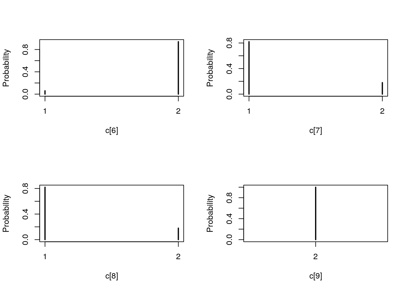
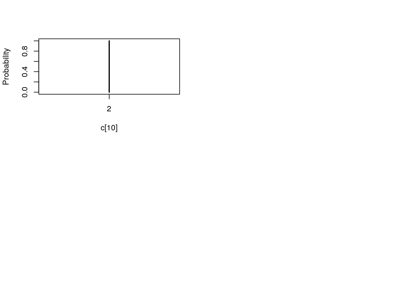
table_pmmh_c <- biips_table(out_pmmh[['c[2:10]']])
par(mfrow = c(2, 2))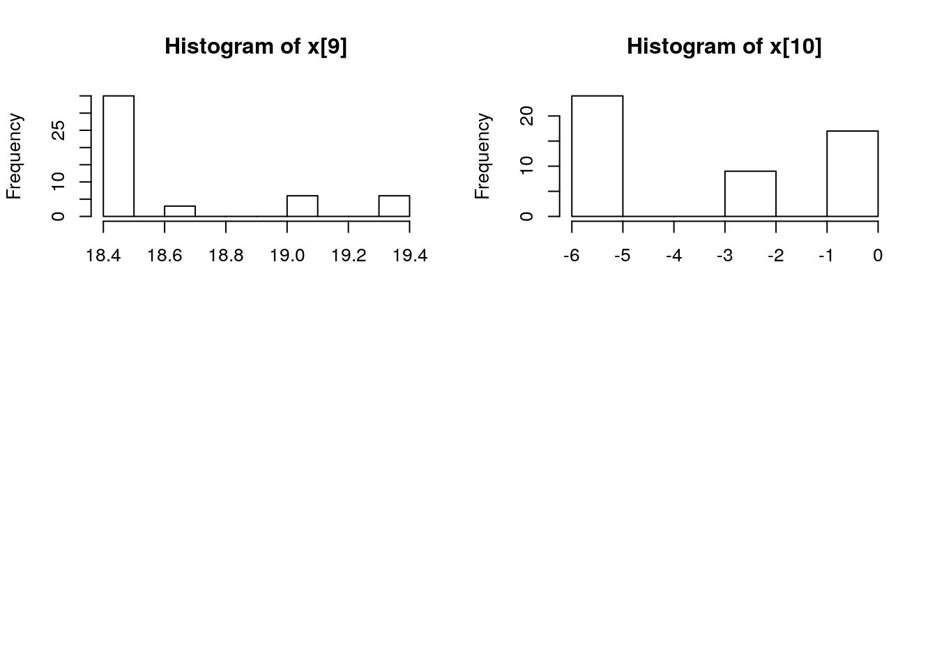
plot(table_pmmh_c)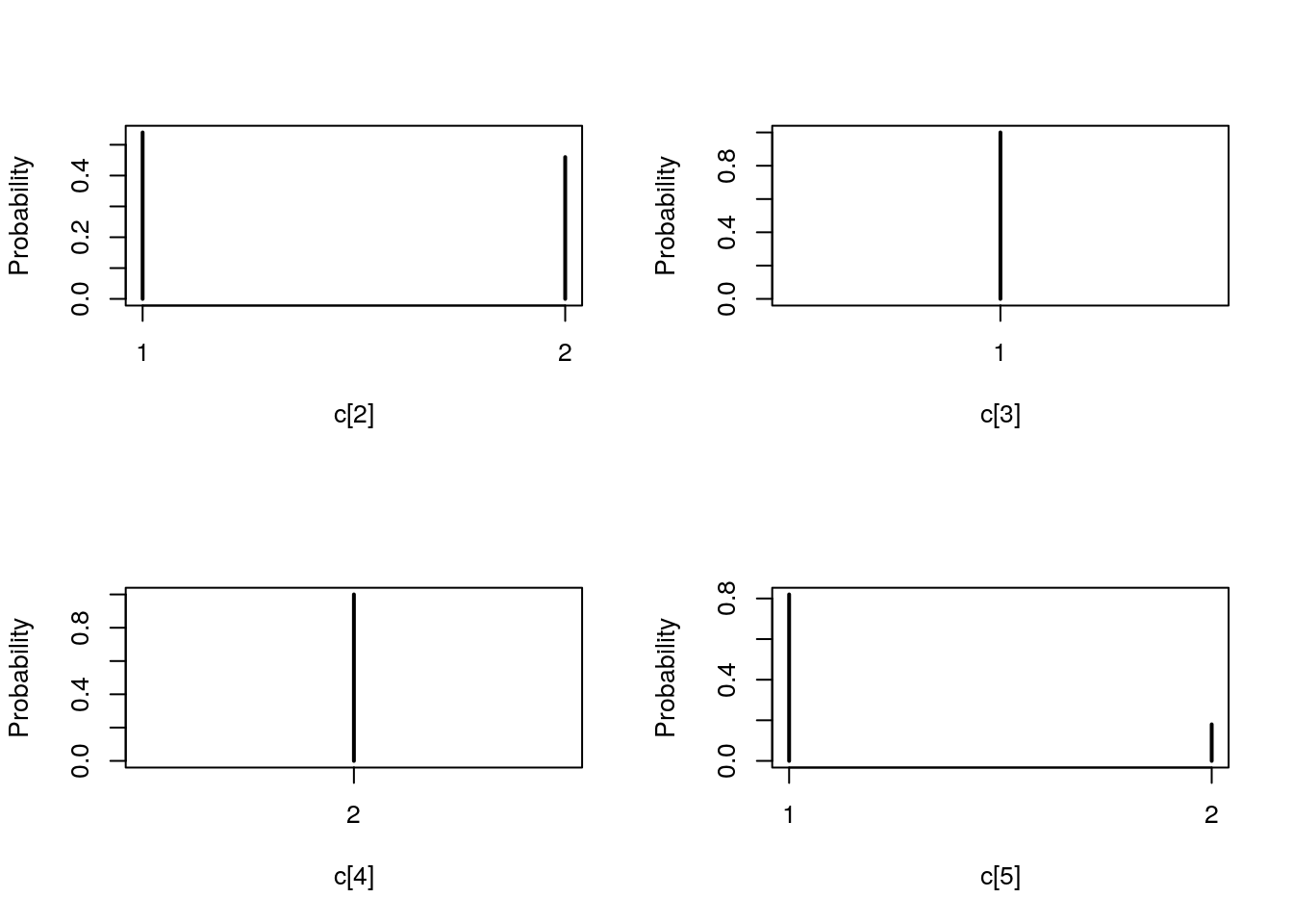
par(mfrow = c(2, 2))
plot(c(out_pmmh_burn$log_marg_like_pen, out_pmmh$log_marg_like_pen), type = 'l',
  col = 'blue', xlab = 'PMMH iteration', ylab = 'log p(y, logtau)')

plot(out_pmmh$logtau[1, ], type = 'l', col = 'blue',
     xlab = 'PMMH iteration', ylab = 'logtau')
points(0, model$data()$logtau_true, pch = 17, col = 'green')

plot(dens_pmmh_lt, col = 'blue', ylab = 'posterior density')
points(model$data()$logtau_true, 0, pch = 17, col = 'green')

biips_hist(out_pmmh$logtau, col = 'blue', ylab = 'posterior density')
points(model$data()$logtau_true, 0, pch = 17, col = 'green')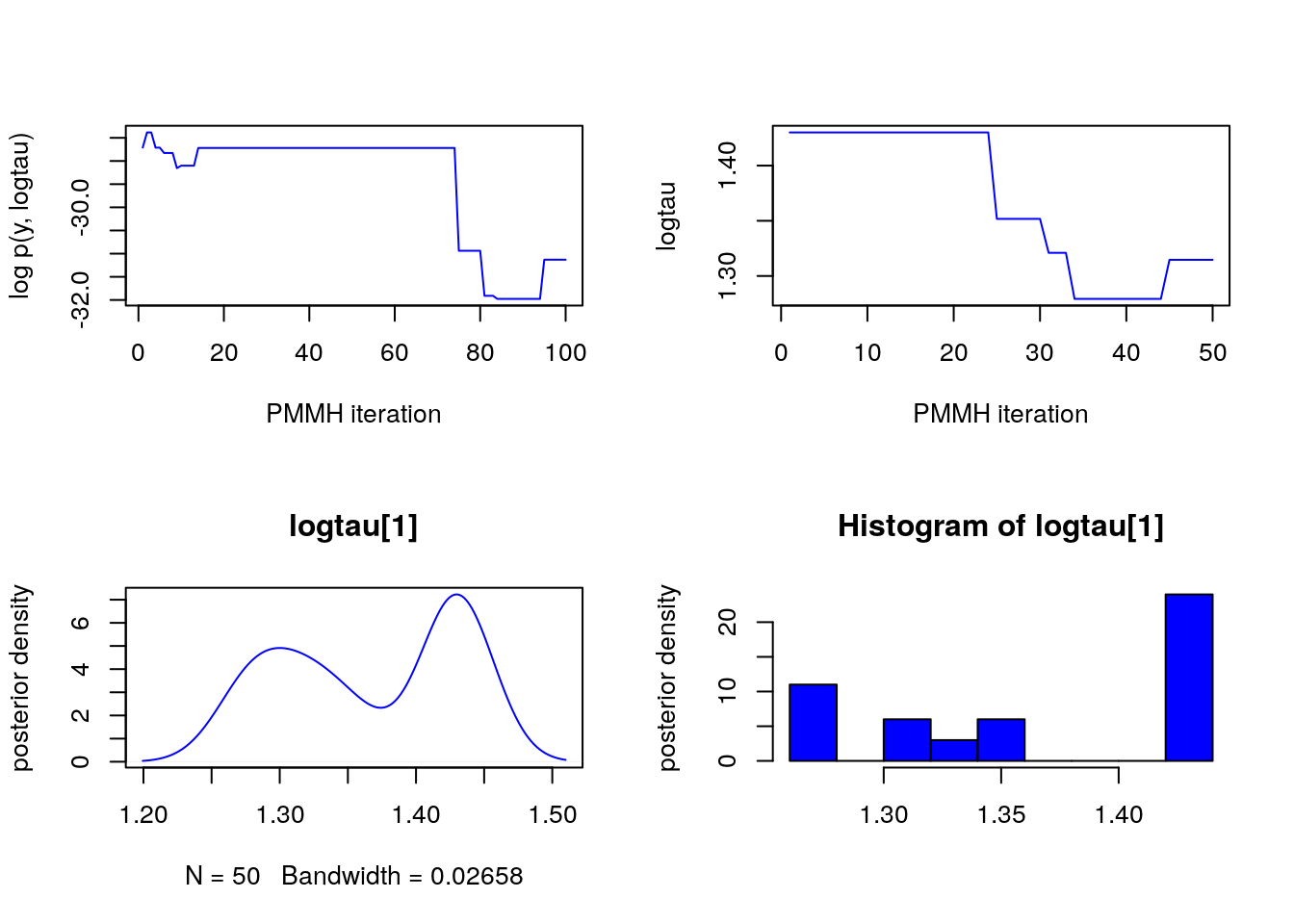
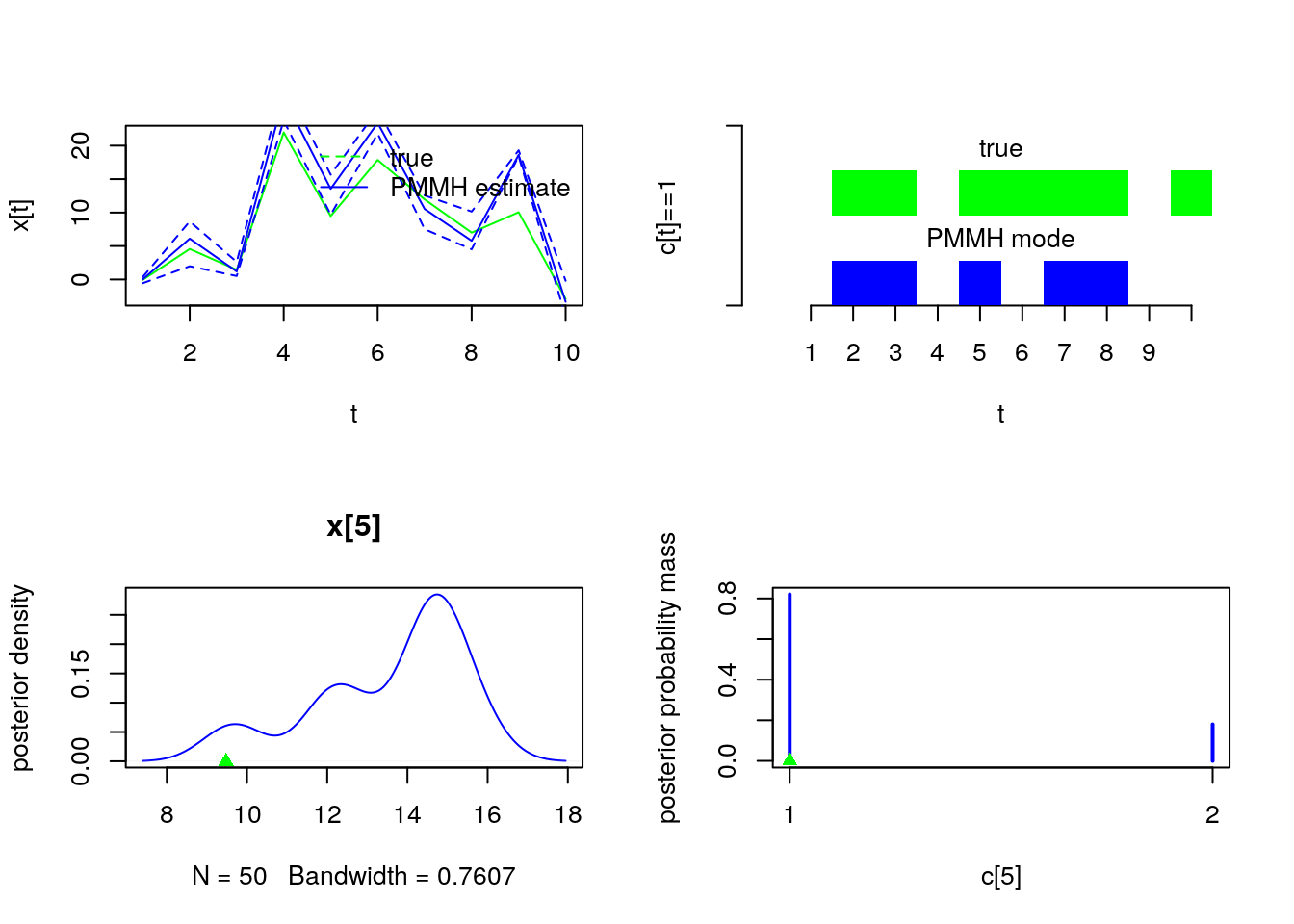
par(mfrow = c(2, 2))
plot(model$data()$x_true, type = 'l', col = 'green', xlab = 't', ylab = 'x[t]')
lines(summ_pmmh_x$mean, col = 'blue')
matlines(matrix(unlist(summ_pmmh_x$quant), data$tmax), lty = 2, col = 'blue')
legend('topright', leg = c('true', 'PMMH estimate'), lty = c(2, 1),
       col = c('green', 'blue'), bty = 'n')

barplot(.5*(model$data()$c_true==1), col = 'green', border = NA, space = 0, offset = 1,
        ylim=c(0,2), xlab='t', ylab='c[t]==1', axes = FALSE)
axis(1, at=1:data$tmax-.5, labels=1:data$tmax)
axis(2, line = 1, at=c(0,2), labels=NA)
text(data$tmax/2, 1.75, 'true')
barplot(.5*c(NA, summ_pmmh_c$mode==1), col = 'blue', border = NA, space = 0, axes = FALSE, add = TRUE)
text(data$tmax/2, .75, 'PMMH mode')

t <- 5
plot(dens_pmmh_x[[t]], col='blue', ylab = 'posterior density')
points(model$data()$x_true[t], 0, pch = 17, col = 'green')

plot(table_pmmh_c[[t-1]], col='blue', ylab = 'posterior probability mass')
points(model$data()$c_true[t], 0, pch = 17, col = 'green')