Matbiips: Tutorial 2
In this tutorial, we consider applying sequential Monte Carlo methods for sensitivity analysis and parameter estimation in a nonlinear non-Gaussian hidden Markov model.
Contents
Statistical model
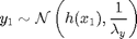
The statistical model is defined as follows.
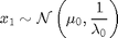
For 
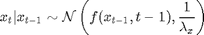
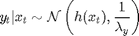
where  denotes the Gaussian distribution of mean
  and covariance matrix
  ,
,  ,
,  ,
,  ,
,  ,
,  . The precision of the observation noise
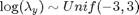
  is also assumed to be unknown. We will assume a uniform prior for
  :
:
Statistical model in BUGS language
We describe the model in BUGS language in the file 'hmm_1d_nonlin.bug':
model_file = 'hmm_1d_nonlin_param.bug'; % BUGS model filename
type(model_file);
var x_true[t_max], x[t_max], y[t_max]

data
{
  #log_prec_y_true ~ dunif(-3, 3)
  prec_y_true <- exp(log_prec_y_true)
  x_true[1] ~ dnorm(mean_x_init, prec_x_init)
  y[1] ~ dnorm(x_true[1]^2/20, prec_y_true)
  for (t in 2:t_max)
  {
    x_true[t] ~ dnorm(0.5*x_true[t-1]+25*x_true[t-1]/(1+x_true[t-1]^2)+8*cos(1.2*(t-1)), prec_x)
    y[t] ~ dnorm(x_true[t]^2/20, prec_y_true)
  }
}

model
{
  log_prec_y ~ dunif(-3, 3)
  prec_y <- exp(log_prec_y)
  x[1] ~ dnorm(mean_x_init, prec_x_init)
  y[1] ~ dnorm(x[1]^2/20, prec_y)
  for (t in 2:t_max)
  {
    x[t] ~ dnorm(0.5*x[t-1]+25*x[t-1]/(1+x[t-1]^2)+8*cos(1.2*(t-1)), prec_x)
    y[t] ~ dnorm(x[t]^2/20, prec_y)
  }
}
Installation of Matbiips
- Download the latest version of Matbiips
- Unzip the archive in some folder
- Add the Matbiips folder to the Matlab search path
matbiips_path = '../../matbiips';
addpath(matbiips_path)
General settings
set(0, 'DefaultAxesFontsize', 14);
set(0, 'Defaultlinelinewidth', 2);
light_blue = [.7, .7, 1];
Set the random numbers generator seed for reproducibility
if isoctave() || verLessThan('matlab', '7.12')
    rand('state', 0)
else
    rng('default')
end
Load model and data
Model parameters
t_max = 20;
mean_x_init = 0;
prec_x_init = 1;
prec_x = 10;
log_prec_y_true = log(1); % True value used to sample the data
data = struct('t_max', t_max, 'prec_x_init', prec_x_init,...
    'prec_x', prec_x, 'log_prec_y_true', log_prec_y_true,...
    'mean_x_init', mean_x_init);
Compile BUGS model and sample data
sample_data = true; % Boolean
model = biips_model(model_file, data, 'sample_data', sample_data); % Create Biips model and sample data
data = model.data;
* Parsing model in: hmm_1d_nonlin_param.bug
* Compiling data graph
  Declaring variables
  Resolving undeclared variables
  Allocating nodes
  Graph size: 280
  Sampling data
  Reading data back into data table
* Compiling model graph
  Declaring variables
  Resolving undeclared variables
  Allocating nodes
  Graph size: 284
Biips Sensitivity analysis with Sequential Monte Carlo
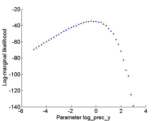
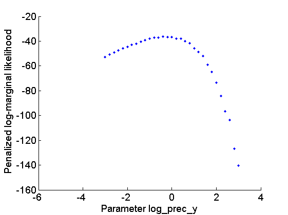
Let now use Biips to provide estimates of the marginal log-likelihood and penalized marginal log-likelihood given various values of the log-precision parameters .
Parameters of the algorithm.
n_part = 100; % Number of particles
param_names = {'log_prec_y'}; % Parameter for which we want to study sensitivity
param_values = {-5:.2:3}; % Range of values
Run sensitivity analysis with SMC
out_sens = biips_smc_sensitivity(model, param_names, param_values, n_part);
* Analyzing sensitivity with 100 particles
  |--------------------------------------------------| 100%
  |**************************************************| 41 iterations in 1.27 s
Plot log-marginal likelihood and penalized log-marginal likelihood
figure('name', 'Log-marginal likelihood');
plot(param_values{1}, out_sens.log_marg_like, '.')
xlabel('Parameter log\_prec\_y')
ylabel('Log-marginal likelihood')
box off

figure('name', 'Penalized log-marginal likelihood');
plot(param_values{1}, out_sens.log_marg_like_pen, '.')
xlabel('Parameter log\_prec\_y')
ylabel('Penalized log-marginal likelihood')
box off
Biips Particle Marginal Metropolis-Hastings
We now use Biips to run a Particle Marginal Metropolis-Hastings in order to obtain posterior MCMC samples of the parameter and the variables  .
.
Parameters of the PMMH.
param_names indicates the parameters to be sampled using a random walk Metroplis-Hastings step. For all the other variables, Biips will use a sequential Monte Carlo as proposal.
n_burn = 2000; % nb of burn-in/adaptation iterations
n_iter = 2000; % nb of iterations after burn-in
thin = 1; % thinning of MCMC outputs
n_part = 50; % nb of particles for the SMC
var_name = 'log_prec_y';
param_names = {var_name}; % name of the variables updated with MCMC (others are updated with SMC)
latent_names = {'x'}; % name of the variables updated with SMC and that need to be monitored
Init PMMH
obj_pmmh = biips_pmmh_init(model, param_names, 'inits', {-2},...
    'latent_names', latent_names); % creates a pmmh object
* Initializing PMMH
Run PMMH
obj_pmmh = biips_pmmh_update(obj_pmmh, n_burn, n_part); % adaptation and burn-in iterations
[obj_pmmh, out_pmmh, log_marg_like_pen, log_marg_like, stats_pmmh] = biips_pmmh_samples(obj_pmmh, n_iter, n_part,...
    'thin', thin); % samples
* Adapting PMMH with 50 particles
  |--------------------------------------------------| 100%
  |++++++++++++++++++++++++++++++++++++++++++++++++++| 2000 iterations in 15.14 s
* Generating 2000 PMMH samples with 50 particles
  |--------------------------------------------------| 100%
  |**************************************************| 2000 iterations in 14.09 s
Some summary statistics
summ_pmmh = biips_summary(out_pmmh, 'probs', [.025, .975]);
Compute kernel density estimates
kde_pmmh = biips_density(out_pmmh);
Posterior mean and credible interval of the parameter
summ_param = getfield(summ_pmmh, var_name);
fprintf('Posterior mean of %s: %.1f\n', var_name, summ_param.mean);
fprintf('95%% credible interval of %s: [%.1f, %.1f]\n', var_name, ...
    summ_param.quant{1}, summ_param.quant{2});
Posterior mean of log_prec_y: -0.4
95% credible interval of log_prec_y: [-1.2, 0.4]
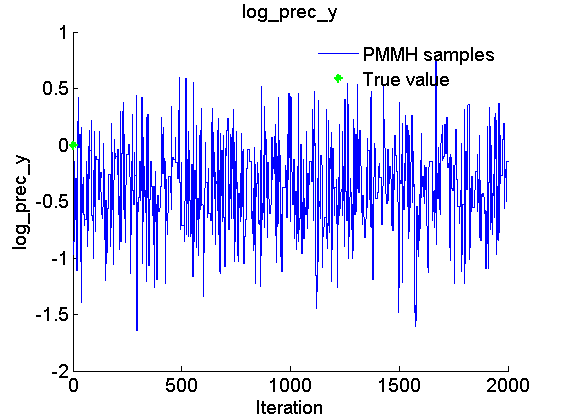
Trace of MCMC samples for the parameter
figure('name', 'PMMH: Trace samples parameter')
samples_param = getfield(out_pmmh, var_name);
param_lab = 'log\_prec\_y';
plot(samples_param, 'linewidth', 1)
hold on
plot(0, data.log_prec_y_true, '*g');
xlabel('Iteration')
ylabel(param_lab)
title(param_lab)
legend({'PMMH samples', 'True value'})
legend boxoff
box off
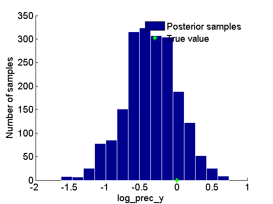
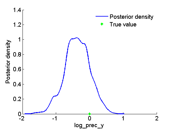
Histogram and kde estimate of the posterior for the parameter
figure('name', 'PMMH: Histogram posterior parameter')
hist(samples_param, 15)
h = findobj(gca, 'Type', 'patch');
set(h, 'EdgeColor', 'w')
hold on
plot(data.log_prec_y_true, 0, '*g');
xlabel(param_lab)
ylabel('Number of samples')
legend({'Posterior samples', 'True value'})
legend boxoff
box off

figure('name', 'PMMH: KDE estimate posterior parameter')
kde_param = getfield(kde_pmmh, var_name);
plot(kde_param.x, kde_param.f);
hold on
plot(data.log_prec_y_true, 0, '*g');
xlabel(param_lab);
ylabel('Posterior density');
legend({'Posterior density', 'True value'})
legend boxoff
box off
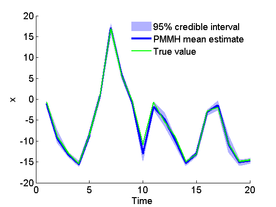
Posterior mean and quantiles for x
figure('name', 'PMMH: Posterior mean and quantiles')
x_pmmh_mean = summ_pmmh.x.mean;
x_pmmh_quant = summ_pmmh.x.quant;
h = fill([1:t_max, t_max:-1:1], [x_pmmh_quant{1}; flipud(x_pmmh_quant{2})], 0);
set(h, 'edgecolor', 'none', 'facecolor', light_blue)
hold on
plot(1:t_max, x_pmmh_mean, 'linewidth', 3)
plot(1:t_max, data.x_true, 'g')
xlabel('Time')
ylabel('x')
legend({'95% credible interval', 'PMMH mean estimate', 'True value'})
box off
legend boxoff
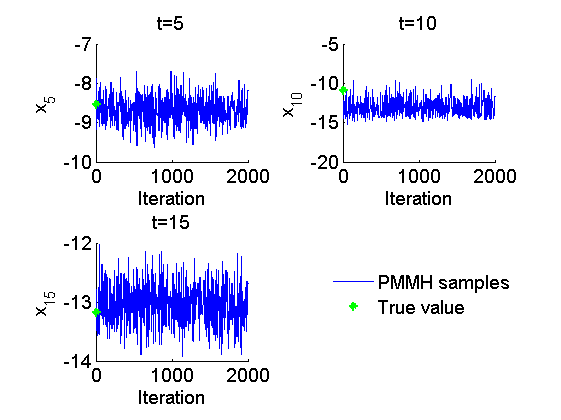
Trace of MCMC samples for x
figure('name', 'PMMH: Trace samples x')
time_index = [5, 10, 15];
for k=1:numel(time_index)
    tk = time_index(k);
    subplot(2, 2, k)
    plot(out_pmmh.x(tk, :), 'linewidth', 1)
    hold on
    plot(0, data.x_true(tk), '*g');
    xlabel('Iteration')
    ylabel(['x_{', num2str(tk), '}'])
    title(['t=', num2str(tk)]);
    box off
end
h = legend({'PMMH samples', 'True value'});
set(h, 'position', [0.7, 0.25, .1, .1])
legend boxoff
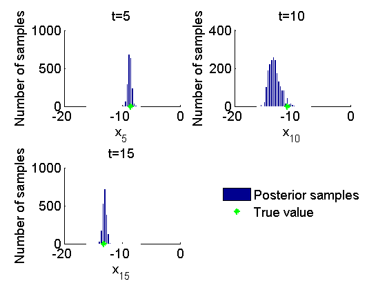
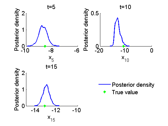
Histogram and kernel density estimate of posteriors of x
figure('name', 'PMMH: Histograms marginal posteriors')
for k=1:numel(time_index)
    tk = time_index(k);
    subplot(2, 2, k)
    hist(out_pmmh.x(tk, :), -16:.3:-7);
    h = findobj(gca, 'Type', 'patch');
    set(h, 'EdgeColor', 'w')
    hold on
    plot(data.x_true(tk), 0, '*g');
    xlabel(['x_{', num2str(tk), '}']);
    ylabel('Number of samples');
    title(['t=', num2str(tk)]);
    box off
end
h = legend({'Posterior samples', 'True value'});
set(h, 'position', [0.7, 0.25, .1, .1])
legend boxoff

figure('name', 'PMMH: KDE estimates marginal posteriors')
for k=1:numel(time_index)
    tk = time_index(k);
    subplot(2, 2, k)
    plot(kde_pmmh.x(tk).x, kde_pmmh.x(tk).f);
    hold on
    plot(data.x_true(tk), 0, '*g');
    xlabel(['x_{', num2str(tk), '}']);
    ylabel('Posterior density');
    title(['t=', num2str(tk)]);
    box off
end
h = legend({'Posterior density', 'True value'});
set(h, 'position', [0.7, 0.25, .1, .1]);
legend boxoff
Clear model
biips_clear()