Matbiips: Tutorial 1

In this tutorial, we consider applying sequential Monte Carlo methods for Bayesian inference in a nonlinear non-Gaussian hidden Markov model.

Statistical model
Statistical model in BUGS language
Installation of Matbiips
General settings
Load model and data
Biips Sequential Monte Carlo
Biips Particle Independent Metropolis-Hastings
Clear model

Statistical model

The statistical model is defined as follows.

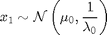
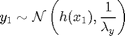
$x_1\sim \mathcal N\left (\mu_0, \frac{1}{\lambda_0}\right )$

$y_1\sim \mathcal N\left (h(x_1), \frac{1}{\lambda_y}\right )$

For $t=2:t_{max}$

$x_t|x_{t-1} \sim \mathcal N\left ( f(x_{t-1},t-1), \frac{1}{\lambda_x}\right )$

$y_t|x_t \sim \mathcal N\left ( h(x_{t}), \frac{1}{\lambda_y}\right )$

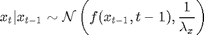
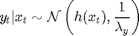
where $\mathcal N\left (m, S\right )$ denotes the Gaussian distribution of mean $m$ and covariance matrix $S$ , $h(x)=x^2/20$ , $f(x,t-1)=0.5 x+25 x/(1+x^2)+8 \cos(1.2 (t-1))$ , $\mu_0=0$ , $\lambda_0 = 5$ , $\lambda_x = 0.1$ and $\lambda_y=1$ .

Statistical model in BUGS language

We describe the model in BUGS language in the file 'hmm_1d_nonlin.bug':

model_file = 'hmm_1d_nonlin.bug'; % BUGS model filename
type(model_file);

var x_true[t_max], x[t_max], y[t_max]

data
{
  x_true[1] ~ dnorm(mean_x_init, prec_x_init)
  y[1] ~ dnorm(x_true[1]^2/20, prec_y)
  for (t in 2:t_max)
  {
    x_true[t] ~ dnorm(0.5*x_true[t-1]+25*x_true[t-1]/(1+x_true[t-1]^2)+8*cos(1.2*(t-1)), prec_x)
    y[t] ~ dnorm(x_true[t]^2/20, prec_y)
  }
}


model
{
  x[1] ~ dnorm(mean_x_init, prec_x_init)
  y[1] ~ dnorm(x[1]^2/20, prec_y)
  for (t in 2:t_max)
  {
    x[t] ~ dnorm(0.5*x[t-1]+25*x[t-1]/(1+x[t-1]^2)+8*cos(1.2*(t-1)), prec_x)
    y[t] ~ dnorm(x[t]^2/20, prec_y)
  }
}

Installation of Matbiips

Download the latest version of Matbiips
Unzip the archive in some folder
Add the Matbiips folder to the Matlab search path

matbiips_path = '../../matbiips';
addpath(matbiips_path)

General settings

set(0, 'defaultaxesfontsize', 14);
set(0, 'defaultlinelinewidth', 2);
light_blue = [.7, .7, 1];
light_red = [1, .7, .7];

Set the random numbers generator seed for reproducibility

if isoctave() || verLessThan('matlab', '7.12')
    rand('state', 0)
else
    rng('default')
end

Load model and data

Model parameters

t_max = 20;
mean_x_init = 0;
prec_x_init = 1/5;
prec_x = 1/10;
prec_y = 1;
data = struct('t_max', t_max, 'prec_x_init', prec_x_init,...
    'prec_x', prec_x, 'prec_y', prec_y, 'mean_x_init', mean_x_init);

Compile BUGS model and sample data

sample_data = true; % Boolean
model = biips_model(model_file, data, 'sample_data', sample_data); % Create Biips model and sample data
data = model.data;

* Parsing model in: hmm_1d_nonlin.bug
* Compiling data graph
  Declaring variables
  Resolving undeclared variables
  Allocating nodes
  Graph size: 279
  Sampling data
  Reading data back into data table
* Compiling model graph
  Declaring variables
  Resolving undeclared variables
  Allocating nodes
  Graph size: 280

Biips Sequential Monte Carlo

Let now use Biips to run a particle filter.

Parameters of the algorithm.

We want to monitor the variable x, and to get the filtering and smoothing particle approximations. The algorithm will use 10000 particles, stratified resampling, with a threshold of 0.5.

n_part = 10000; % Number of particles
variables = {'x'}; % Variables to be monitored
mn_type = 'fs'; rs_type = 'stratified'; rs_thres = 0.5; % Optional parameters

Run SMC

out_smc = biips_smc_samples(model, variables, n_part,...
    'type', mn_type, 'rs_type', rs_type, 'rs_thres', rs_thres);

* Assigning node samplers
* Running SMC forward sampler with 10000 particles
  |--------------------------------------------------| 100%
  |**************************************************| 20 iterations in 2.86 s

Diagnosis of the algorithm

diag_smc = biips_diagnosis(out_smc);

* Diagnosis of variable: x[1:20]
  Filtering: GOOD
  Smoothing: GOOD

The sequence of filtering distributions is automatically chosen by Biips based on the topology of the graphical model, and is returned in the subfield f.conditionals. For this particular example, the sequence of filtering distributions is $\pi(x_{t}|y_{1:t})$ , for $t=1,\ldots,t_{max}$ .

fprintf('Filtering distributions:\n')
for i=1:numel(out_smc.x.f.conditionals)
    fprintf('%i: x[%i] | ', out_smc.x.f.iterations(i), i);
    fprintf('%s,', out_smc.x.f.conditionals{i}{1:end-1});
    fprintf('%s', out_smc.x.f.conditionals{i}{end});
    fprintf('\n')
end

Filtering distributions:
1: x[1] | y[1]
2: x[2] | y[1],y[2]
3: x[3] | y[1],y[2],y[3]
4: x[4] | y[1],y[2],y[3],y[4]
5: x[5] | y[1],y[2],y[3],y[4],y[5]
6: x[6] | y[1],y[2],y[3],y[4],y[5],y[6]
7: x[7] | y[1],y[2],y[3],y[4],y[5],y[6],y[7]
8: x[8] | y[1],y[2],y[3],y[4],y[5],y[6],y[7],y[8]
9: x[9] | y[1],y[2],y[3],y[4],y[5],y[6],y[7],y[8],y[9]
10: x[10] | y[1],y[2],y[3],y[4],y[5],y[6],y[7],y[8],y[9],y[10]
11: x[11] | y[1],y[2],y[3],y[4],y[5],y[6],y[7],y[8],y[9],y[10],y[11]
12: x[12] | y[1],y[2],y[3],y[4],y[5],y[6],y[7],y[8],y[9],y[10],y[11],y[12]
13: x[13] | y[1],y[2],y[3],y[4],y[5],y[6],y[7],y[8],y[9],y[10],y[11],y[12],y[13]
14: x[14] | y[1],y[2],y[3],y[4],y[5],y[6],y[7],y[8],y[9],y[10],y[11],y[12],y[13],y[14]
15: x[15] | y[1],y[2],y[3],y[4],y[5],y[6],y[7],y[8],y[9],y[10],y[11],y[12],y[13],y[14],y[15]
16: x[16] | y[1],y[2],y[3],y[4],y[5],y[6],y[7],y[8],y[9],y[10],y[11],y[12],y[13],y[14],y[15],y[16]
17: x[17] | y[1],y[2],y[3],y[4],y[5],y[6],y[7],y[8],y[9],y[10],y[11],y[12],y[13],y[14],y[15],y[16],y[17]
18: x[18] | y[1],y[2],y[3],y[4],y[5],y[6],y[7],y[8],y[9],y[10],y[11],y[12],y[13],y[14],y[15],y[16],y[17],y[18]
19: x[19] | y[1],y[2],y[3],y[4],y[5],y[6],y[7],y[8],y[9],y[10],y[11],y[12],y[13],y[14],y[15],y[16],y[17],y[18],y[19]
20: x[20] | y[1],y[2],y[3],y[4],y[5],y[6],y[7],y[8],y[9],y[10],y[11],y[12],y[13],y[14],y[15],y[16],y[17],y[18],y[19],y[20]

while the smoothing distributions are $\pi(x_{t}|y_{1:t_{max}})$ , for $t=1,\ldots,t_{max}$ .

fprintf('Smoothing distributions:\n')
for i=1:numel(out_smc.x.s.conditionals)
    fprintf('x[%i] | ', i);
    fprintf('%s,', out_smc.x.s.conditionals{1:end-1});
    fprintf('%s', out_smc.x.s.conditionals{end});
    fprintf('\n')
end

Smoothing distributions:
x[1] | y[1],y[2],y[3],y[4],y[5],y[6],y[7],y[8],y[9],y[10],y[11],y[12],y[13],y[14],y[15],y[16],y[17],y[18],y[19],y[20]
x[2] | y[1],y[2],y[3],y[4],y[5],y[6],y[7],y[8],y[9],y[10],y[11],y[12],y[13],y[14],y[15],y[16],y[17],y[18],y[19],y[20]
x[3] | y[1],y[2],y[3],y[4],y[5],y[6],y[7],y[8],y[9],y[10],y[11],y[12],y[13],y[14],y[15],y[16],y[17],y[18],y[19],y[20]
x[4] | y[1],y[2],y[3],y[4],y[5],y[6],y[7],y[8],y[9],y[10],y[11],y[12],y[13],y[14],y[15],y[16],y[17],y[18],y[19],y[20]
x[5] | y[1],y[2],y[3],y[4],y[5],y[6],y[7],y[8],y[9],y[10],y[11],y[12],y[13],y[14],y[15],y[16],y[17],y[18],y[19],y[20]
x[6] | y[1],y[2],y[3],y[4],y[5],y[6],y[7],y[8],y[9],y[10],y[11],y[12],y[13],y[14],y[15],y[16],y[17],y[18],y[19],y[20]
x[7] | y[1],y[2],y[3],y[4],y[5],y[6],y[7],y[8],y[9],y[10],y[11],y[12],y[13],y[14],y[15],y[16],y[17],y[18],y[19],y[20]
x[8] | y[1],y[2],y[3],y[4],y[5],y[6],y[7],y[8],y[9],y[10],y[11],y[12],y[13],y[14],y[15],y[16],y[17],y[18],y[19],y[20]
x[9] | y[1],y[2],y[3],y[4],y[5],y[6],y[7],y[8],y[9],y[10],y[11],y[12],y[13],y[14],y[15],y[16],y[17],y[18],y[19],y[20]
x[10] | y[1],y[2],y[3],y[4],y[5],y[6],y[7],y[8],y[9],y[10],y[11],y[12],y[13],y[14],y[15],y[16],y[17],y[18],y[19],y[20]
x[11] | y[1],y[2],y[3],y[4],y[5],y[6],y[7],y[8],y[9],y[10],y[11],y[12],y[13],y[14],y[15],y[16],y[17],y[18],y[19],y[20]
x[12] | y[1],y[2],y[3],y[4],y[5],y[6],y[7],y[8],y[9],y[10],y[11],y[12],y[13],y[14],y[15],y[16],y[17],y[18],y[19],y[20]
x[13] | y[1],y[2],y[3],y[4],y[5],y[6],y[7],y[8],y[9],y[10],y[11],y[12],y[13],y[14],y[15],y[16],y[17],y[18],y[19],y[20]
x[14] | y[1],y[2],y[3],y[4],y[5],y[6],y[7],y[8],y[9],y[10],y[11],y[12],y[13],y[14],y[15],y[16],y[17],y[18],y[19],y[20]
x[15] | y[1],y[2],y[3],y[4],y[5],y[6],y[7],y[8],y[9],y[10],y[11],y[12],y[13],y[14],y[15],y[16],y[17],y[18],y[19],y[20]
x[16] | y[1],y[2],y[3],y[4],y[5],y[6],y[7],y[8],y[9],y[10],y[11],y[12],y[13],y[14],y[15],y[16],y[17],y[18],y[19],y[20]
x[17] | y[1],y[2],y[3],y[4],y[5],y[6],y[7],y[8],y[9],y[10],y[11],y[12],y[13],y[14],y[15],y[16],y[17],y[18],y[19],y[20]
x[18] | y[1],y[2],y[3],y[4],y[5],y[6],y[7],y[8],y[9],y[10],y[11],y[12],y[13],y[14],y[15],y[16],y[17],y[18],y[19],y[20]
x[19] | y[1],y[2],y[3],y[4],y[5],y[6],y[7],y[8],y[9],y[10],y[11],y[12],y[13],y[14],y[15],y[16],y[17],y[18],y[19],y[20]
x[20] | y[1],y[2],y[3],y[4],y[5],y[6],y[7],y[8],y[9],y[10],y[11],y[12],y[13],y[14],y[15],y[16],y[17],y[18],y[19],y[20]

Summary statistics

summ_smc = biips_summary(out_smc, 'probs', [.025, .975]);

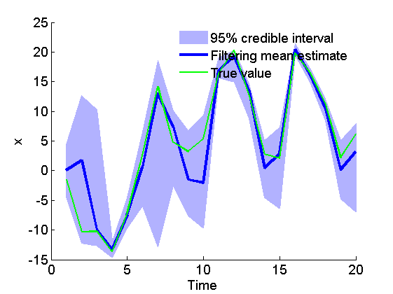
Plot Filtering estimates

figure('name', 'SMC: Filtering estimates')
x_f_mean = summ_smc.x.f.mean;
x_f_quant = summ_smc.x.f.quant;
h = fill([1:t_max, t_max:-1:1], [x_f_quant{1}; flipud(x_f_quant{2})], 0);
set(h, 'edgecolor', 'none', 'facecolor', light_blue)
hold on
plot(1:t_max, x_f_mean, 'linewidth', 3)
plot(1:t_max, data.x_true, 'g')
xlabel('Time')
ylabel('x')
legend({'95% credible interval', 'Filtering mean estimate', 'True value'})
legend boxoff
box off

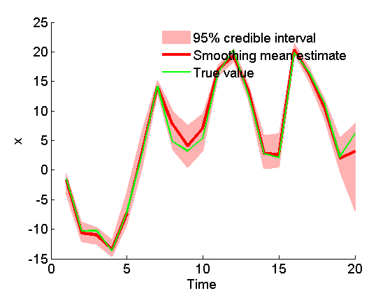
Plot Smoothing estimates

figure('name', 'SMC: Smoothing estimates')
x_s_mean = summ_smc.x.s.mean;
x_s_quant = summ_smc.x.s.quant;
h = fill([1:t_max, t_max:-1:1], [x_s_quant{1}; flipud(x_s_quant{2})], 0);
set(h, 'edgecolor', 'none', 'facecolor', light_red)
hold on
plot(1:t_max, x_s_mean, 'r', 'linewidth', 3)
plot(1:t_max, data.x_true, 'g')
xlabel('Time')
ylabel('x')
legend({'95% credible interval', 'Smoothing mean estimate', 'True value'})
legend boxoff
box off

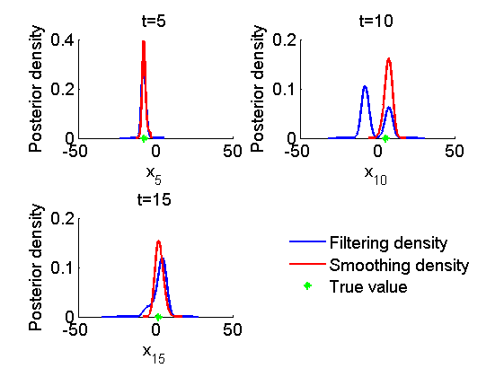
Marginal filtering and smoothing densities

figure('name', 'SMC: Marginal posteriors')
kde_smc = biips_density(out_smc);
time_index = [5, 10, 15];
for k=1:numel(time_index)
    tk = time_index(k);
    subplot(2, 2, k)
    plot(kde_smc.x.f(tk).x, kde_smc.x.f(tk).f);
    hold on
    plot(kde_smc.x.s(tk).x, kde_smc.x.s(tk).f, 'r');
    plot(data.x_true(tk), 0, '*g');
    xlabel(['x_{', num2str(tk), '}']);
    ylabel('Posterior density');
    title(['t=', num2str(tk)]);
    box off
end
h = legend({'Filtering density', 'Smoothing density', 'True value'});
set(h, 'position', [0.7, 0.25, .1, .1])
legend boxoff

Biips Particle Independent Metropolis-Hastings

We now use Biips to run a Particle Independent Metropolis-Hastings.

Parameters of the PIMH

n_burn = 500;
n_iter = 500;
thin = 1;
n_part = 100;

Run PIMH

obj_pimh = biips_pimh_init(model, variables);
obj_pimh = biips_pimh_update(obj_pimh, n_burn, n_part); % burn-in iterations
[obj_pimh, samples_pimh, log_marg_like_pimh] = biips_pimh_samples(obj_pimh,...
    n_iter, n_part, 'thin', thin);

* Initializing PIMH
* Updating PIMH with 100 particles
  |--------------------------------------------------| 100%
  |**************************************************| 500 iterations in 7.03 s
* Generating PIMH samples with 100 particles
  |--------------------------------------------------| 100%
  |**************************************************| 500 iterations in 6.73 s

Some summary statistics

summ_pimh = biips_summary(samples_pimh, 'probs', [.025, .975]);

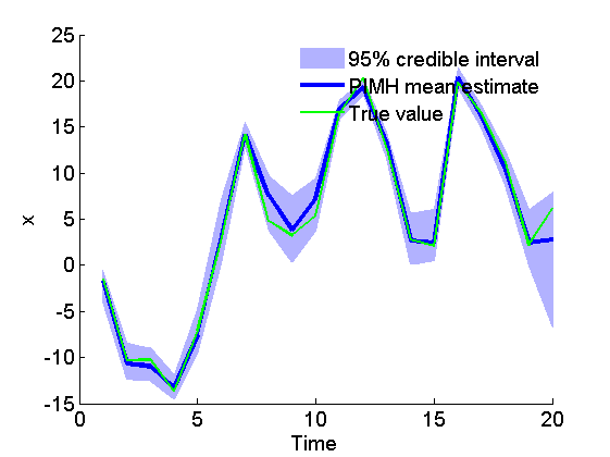
Posterior mean and quantiles

figure('name', 'PIMH: Posterior mean and quantiles')
x_pimh_mean = summ_pimh.x.mean;
x_pimh_quant = summ_pimh.x.quant;
h = fill([1:t_max, t_max:-1:1], [x_pimh_quant{1}; flipud(x_pimh_quant{2})], 0);
set(h, 'edgecolor', 'none', 'facecolor', light_blue)
hold on
plot(1:t_max, x_pimh_mean, 'linewidth', 3)
plot(1:t_max, data.x_true, 'g')
xlabel('Time')
ylabel('x')
legend({'95% credible interval', 'PIMH mean estimate', 'True value'})
legend boxoff
box off

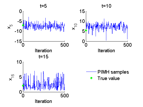
Trace of MCMC samples

figure('name', 'PIMH: Trace samples')
time_index = [5, 10, 15];
for k=1:numel(time_index)
    tk = time_index(k);
    subplot(2, 2, k)
    plot(samples_pimh.x(tk, :), 'linewidth', 1)
    hold on
    plot(0, data.x_true(tk), '*g');
    xlabel('Iteration')
    ylabel(['x_{', num2str(tk), '}'])
    title(['t=', num2str(tk)]);
    box off
end
h = legend({'PIMH samples', 'True value'});
set(h, 'position', [0.7, 0.25, .1, .1])
legend boxoff

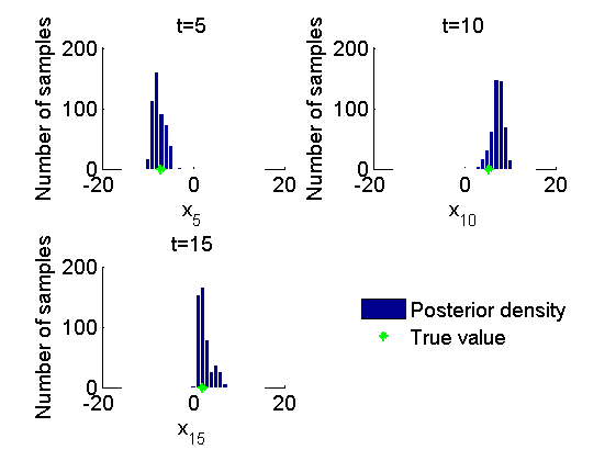
Histograms of posteriors

figure('name', 'PIMH: Histograms marginal posteriors')
for k=1:numel(time_index)
    tk = time_index(k);
    subplot(2, 2, k)
    hist(samples_pimh.x(tk, :), -15:1:15);
    h = findobj(gca, 'Type', 'patch');
    set(h, 'EdgeColor', 'w')
    hold on
    plot(data.x_true(tk), 0, '*g');
    xlabel(['x_{', num2str(tk), '}']);
    ylabel('Number of samples');
    title(['t=', num2str(tk)]);
    box off
end
h = legend({'Posterior density', 'True value'});
set(h, 'position', [0.7, 0.25, .1, .1])
legend boxoff

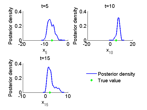
Kernel density estimates of posteriors

figure('name', 'PIMH: KDE estimates marginal posteriors')
kde_pimh = biips_density(samples_pimh);
for k=1:numel(time_index)
    tk = time_index(k);
    subplot(2, 2, k)
    plot(kde_pimh.x(tk).x, kde_pimh.x(tk).f);
    hold on
    plot(data.x_true(tk), 0, '*g');
    xlabel(['x_{', num2str(tk), '}']);
    ylabel('Posterior density');
    title(['t=', num2str(tk)]);
    box off
end
h = legend({'Posterior density', 'True value'});
set(h, 'position', [0.7, 0.25, .1, .1])
legend boxoff

Clear model

biips_clear()