Matbiips example: Switching stochastic volatility with estimation of static parameters
In this example, we consider the Markov switching stochastic volatility model with parameter estimation.
Reference: C.M. Carvalho and H.F. Lopes. Simulation-based sequential analysis of Markov switching stochastic volatility models. Computational Statistics and Data analysis (2007) 4526-4542.
Contents
Statistical model
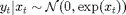
Let  be the response variable and
  the unobserved log-volatility of . The stochastic volatility model is defined as follows for

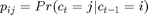
The regime variables  follow a two-state Markov process with transition probabilities
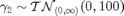
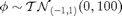
We assume the following priors over the parameters  :
:


 denotes the normal distribution of mean
  and variance
  .
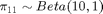
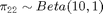
.  denotes the truncated normal distribution of mean and variance .
Statistical model in BUGS language
Content of the file 'switch_stoch_volatility_param.bug':
model_file = 'switch_stoch_volatility_param.bug'; % BUGS model filename
type(model_file);
# Switching Stochastic Volatility Model
# Reference: C.M. Carvalho and H.F. Lopes. Simulation-based sequential analysis of Markov switching
# stochastic volatility models. Computational Statistics and Data analysis (2007) 4526-4542.

var y[t_max],x[t_max],prec_y[t_max],mu[t_max],mu_true[t_max],alpha[2],gamma[2],c[t_max],c_true[t_max],pi[2,2]

data
{
  c_true[1] ~ dcat(pi_true[1,])
  mu_true[1] <- alpha_true[1] * (c_true[1]==1) + alpha_true[2]*(c_true[1]==2)
  x_true[1] ~ dnorm(mu_true[1], 1/sigma_true^2) T(-500,500)
  prec_y_true[1] <- exp(-x_true[1])
  y[1] ~ dnorm(0, prec_y_true[1])
  for (t in 2:t_max)
  {
    c_true[t] ~ dcat(ifelse(c_true[t-1]==1,pi_true[1,],pi_true[2,]))
    mu_true[t] <- alpha_true[1] * (c_true[t]==1) + alpha_true[2] * (c_true[t]==2) + phi_true * x_true[t-1];
    x_true[t] ~ dnorm(mu_true[t], 1/sigma_true^2) T(-500,500)
    prec_y_true[t] <- exp(-x_true[t])
    y[t] ~ dnorm(0, prec_y_true[t])
  }
}

model
{
  gamma[1] ~ dnorm(0, 1/100)
  gamma[2] ~ dnorm(0, 1/100) T(0,)
  alpha[1] <- gamma[1]
  alpha[2] <- gamma[1] + gamma[2]
  phi ~ dnorm(0, 1/100) T(-1,1)
  tau ~ dgamma(2.001, 1)
  sigma <- 1/sqrt(tau)
  pi[1,1] ~ dbeta(10, 1)
  pi[1,2] <- 1 - pi[1,1]
  pi[2,2] ~ dbeta(10, 1)
  pi[2,1] <- 1 - pi[2,2]


  c[1] ~ dcat(pi[1,])
  mu[1] <- alpha[1] * (c[1]==1) + alpha[2] * (c[1]==2)
  x[1] ~ dnorm(mu[1], 1/sigma^2) T(-500,500)
  prec_y[1] <- exp(-x[1])
  y[1] ~ dnorm(0, prec_y[1])
  for (t in 2:t_max)
  {
    c[t] ~ dcat(ifelse(c[t-1]==1, pi[1,], pi[2,]))
    mu[t] <- alpha[1] * (c[t]==1) + alpha[2] * (c[t]==2) + phi * x[t-1]
    x[t] ~ dnorm(mu[t], 1/sigma^2) T(-500,500)
    prec_y[t] <- exp(-x[t])
    y[t] ~ dnorm(0, prec_y[t])
  }
}
Installation of Matbiips
- Download the latest version of Matbiips
- Unzip the archive in some folder
- Add the Matbiips folder to the Matlab search path
matbiips_path = '../../matbiips';
addpath(matbiips_path)
General settings
set(0, 'DefaultAxesFontsize', 16);
set(0, 'Defaultlinelinewidth', 2);
set(0, 'DefaultLineMarkerSize', 8);
light_blue = [.7, .7, 1];
light_red = [1, .7, .7];
light_green = [.7, 1, .7];
light_gray = [.9,.9,.9];

% Set the random numbers generator seed for reproducibility
if isoctave() || verLessThan('matlab', '7.12')
    rand('state', 0)
else
    rng('default')
end
Load model and load or simulate data
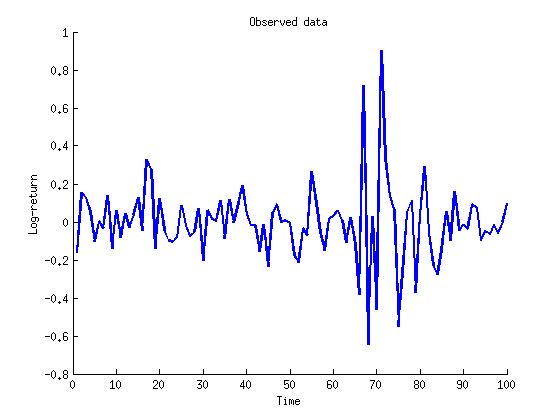
sample_data = true; % Simulated data or SP500 data
t_max = 100;

if ~sample_data
    % Load the data
    T = readtable('SP500.csv', 'delimiter', ';');
    y = diff(log(T.Close(end:-1:1)));
    SP500_date_str = T.Date(end:-1:2);

    ind = 1:t_max;
    y = y(ind);
    SP500_date_str = SP500_date_str(ind);

    SP500_date_num = datenum(SP500_date_str);
end
Model parameters
if ~sample_data
    data = struct('t_max', t_max, 'y', y);
else
    sigma_true = .4;
    alpha_true = [-2.5; -1];
    phi_true = .5;
    pi11 = .9;
    pi22 = .9;
    pi_true = [pi11, 1-pi11;
        1-pi22, pi22];

    data = struct('t_max', t_max, 'sigma_true', sigma_true,...
        'alpha_true', alpha_true, 'phi_true', phi_true, 'pi_true', pi_true);
end
Compile BUGS model and sample data if simulated data
model = biips_model(model_file, data, 'sample_data', sample_data);
data = model.data;
Plot the data
figure('name', 'Log-returns')
if sample_data
    plot(1:t_max, data.y)
    title('Observed data')
    xlabel('Time')
else
    plot(SP500_date_num, data.y)
    title('Observed data: S&P 500')
    datetick('x', 'mmmyyyy', 'keepticks')
    xlabel('Date')
end
ylabel('Log-return')
box off
saveas(gca, 'switch_stoch_param_obs', 'epsc2')
saveas(gca, 'switch_stoch_param_obs', 'png')
Biips Particle Marginal Metropolis-Hastings
We now use Biips to run a Particle Marginal Metropolis-Hastings in order to obtain posterior MCMC samples of the parameters  ,
,  ,
,  ,
,  , and of the variables
  . Note: We use below a reduced number of MCMC iterations to have reasonable running times. But the obtained samples are obviously very correlated, and the number of iterations should be set to a higher value, and proper convergence tests should be used.
Parameters of the PMMH
n_burn = 2000; % nb of burn-in/adaptation iterations
n_iter = 40000; % nb of iterations after burn-in
thin = 10; % thinning of MCMC outputs
n_part = 50; % nb of particles for the SMC

param_names = {'gamma[1]', 'gamma[2]', 'phi', 'tau', 'pi[1,1]', 'pi[2,2]'}; % name of the variables updated with MCMC (others are updated with SMC)
latent_names = {'x', 'c', 'alpha[1]', 'alpha[2]', 'sigma'}; % name of the variables updated with SMC and that need to be monitored
Init PMMH
inits = {-1, 1, .5, 10, .8, .8};
obj_pmmh = biips_pmmh_init(model, param_names, 'inits', inits, 'latent_names', latent_names); % creates a pmmh object
* Initializing PMMH
Run PMMH
obj_pmmh  = biips_pmmh_update(obj_pmmh, n_burn, n_part); % adaptation and burn-in iterations

[obj_pmmh, out_pmmh, log_marg_like_pen, log_marg_like] =...
    biips_pmmh_samples(obj_pmmh, n_iter, n_part, 'thin', thin); % Samples
* Adapting PMMH with 50 particles
  |--------------------------------------------------| 100%
  |++++++++++++++++++++++++++++++++++++++++++++++++++| 2000 iterations in 149.60 s
* Generating 4000 PMMH samples with 50 particles
  |--------------------------------------------------| 100%
  |**************************************************| 40000 iterations in 2815.84 s
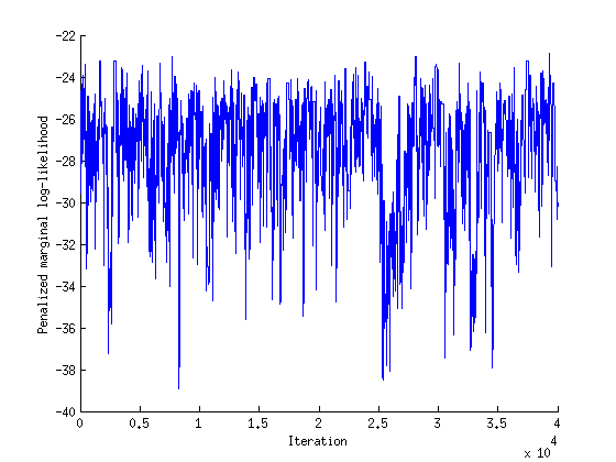
Penalized marginal log-likelihood
figure('name', 'PMMH: Penalized marginal log-likelihood')
iter = thin:thin:n_iter;
plot(iter, log_marg_like_pen, 'linewidth', 1)
xlabel('Iteration')
ylabel('Penalized marginal log-likelihood')
box off
saveas(gca, 'switch_stoch_param_pmll', 'epsc2')
saveas(gca, 'switch_stoch_param_pmll', 'png')
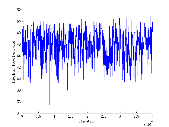
Marginal log-likelihood
figure('name', 'PMMH: Marginal log-likelihood')
iter = thin:thin:n_iter;
plot(iter, log_marg_like, 'linewidth', 1)
xlabel('Iteration')
ylabel('Marginal log-likelihood')
box off
saveas(gca, 'switch_stoch_param_mll', 'epsc2')
saveas(gca, 'switch_stoch_param_mll', 'png')
Some summary statistics
summ_pmmh = biips_summary(out_pmmh, 'probs', [.025, .975]);
Compute kernel density estimates
kde_pmmh = biips_density(out_pmmh);
Compute probability mass function estimates of the discrete marginal variables c[t]
table_c = biips_table(out_pmmh.c);
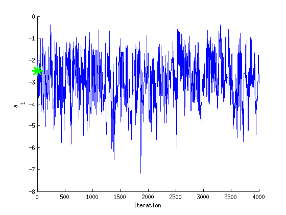
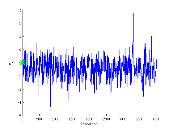
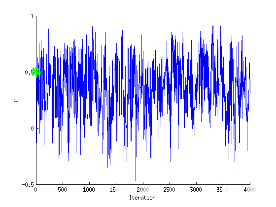
param_plot = {'alpha[1]', 'alpha[2]', 'phi', 'sigma', 'pi[1,1]', 'pi[2,2]'};
param_lab = {'\alpha_1', '\alpha_2', '\phi', '\sigma', '\pi_{11}', '\pi_{22}'};
if sample_data
param_true = [alpha_true', phi_true, sigma_true, pi11, pi22];
end
Posterior mean, MAP and credible interval of the parameters
[~, ind_map] = max(log_marg_like_pen);
[~, ind_mle] = max(log_marg_like);
for i=1:numel(param_plot)
    summ_param = getfield(summ_pmmh, param_plot{i});
    out_param = getfield(out_pmmh, param_plot{i});
    fprintf('Posterior mean of %s: %.3f\n', param_plot{i}, summ_param.mean);
    fprintf('95%% credible interval of %s: [%.3f, %.3f]\n',...
        param_plot{i}, summ_param.quant{1}, summ_param.quant{2});
    fprintf('MAP of %s: %.3f\n', param_plot{i}, out_param(ind_map));
    fprintf('MLE of %s: %.3f\n', param_plot{i}, out_param(ind_mle));
end
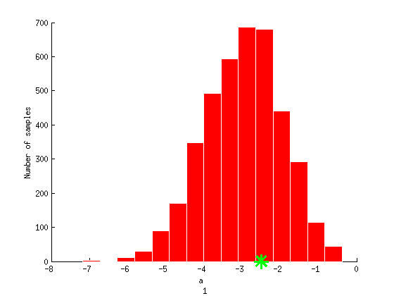
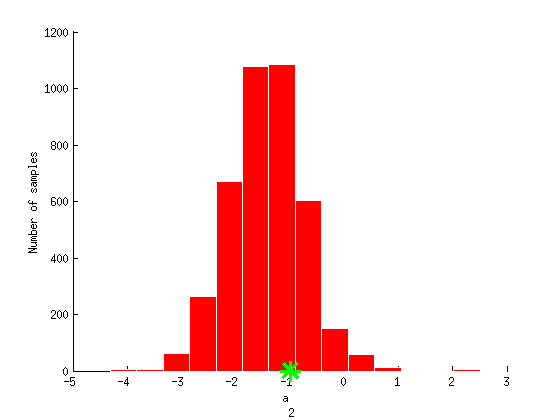
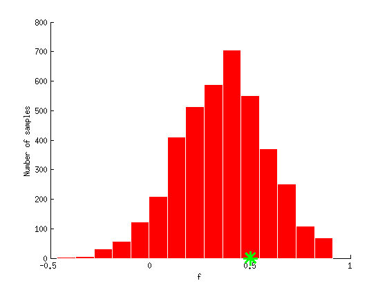
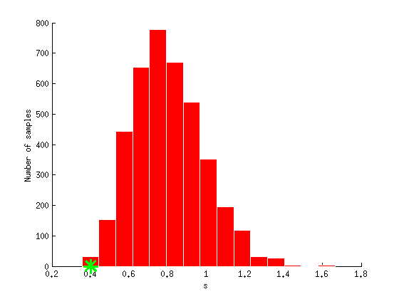
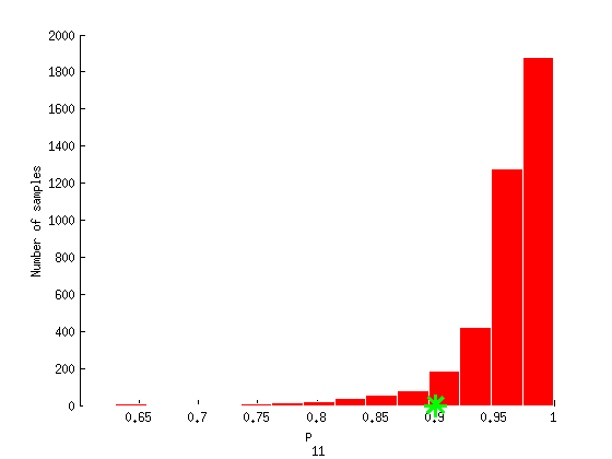
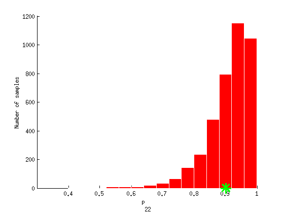
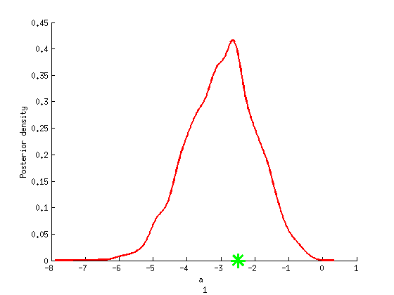
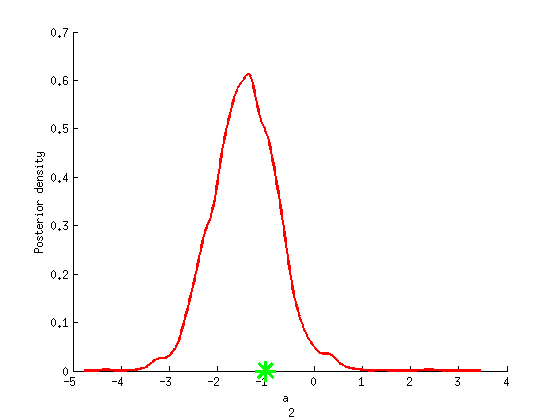
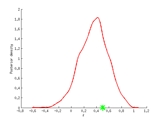
Posterior mean of alpha[1]: -2.979
95% credible interval of alpha[1]: [-4.934, -1.073]
MAP of alpha[1]: -4.143
MLE of alpha[1]: -4.143
Posterior mean of alpha[2]: -1.431
95% credible interval of alpha[2]: [-2.755, -0.036]
MAP of alpha[2]: -2.004
MLE of alpha[2]: -2.004
Posterior mean of phi: 0.358
95% credible interval of phi: [-0.093, 0.786]
MAP of phi: 0.125
MLE of phi: 0.125
Posterior mean of sigma: 0.803
95% credible interval of sigma: [0.485, 1.202]
MAP of sigma: 0.803
MLE of sigma: 0.803
Posterior mean of pi[1,1]: 0.961
95% credible interval of pi[1,1]: [0.833, 0.998]
MAP of pi[1,1]: 0.991
MLE of pi[1,1]: 0.991
Posterior mean of pi[2,2]: 0.911
95% credible interval of pi[2,2]: [0.744, 0.994]
MAP of pi[2,2]: 0.949
MLE of pi[2,2]: 0.949
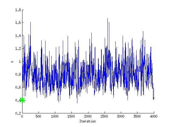
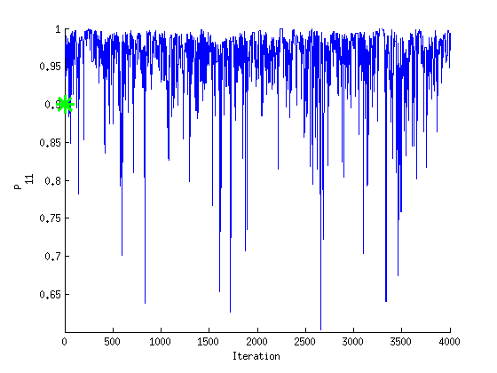
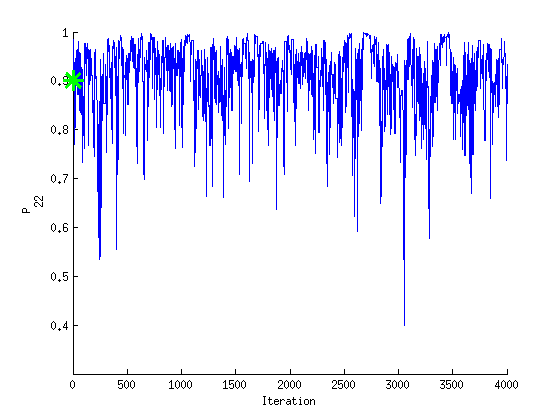
Trace of MCMC samples for the parameters
for k=1:numel(param_plot)
    figure('name', 'PMMH: Trace samples parameter')
    samples_param = getfield(out_pmmh, param_plot{k});
    plot(samples_param, 'linewidth', 1)
    if sample_data
        hold on
        plot(0, param_true(k), '*g', 'linewidth', 3, 'markersize', 16);
    end
    xlabel('Iteration', 'fontsize', 24)
    ylabel(param_lab{k}, 'fontsize', 24)
    box off
%     title(param_lab{k})
    saveas(gca, ['switch_stoch_param_trace', num2str(k)], 'epsc2')
    saveas(gca, ['switch_stoch_param_trace', num2str(k)], 'png')
end
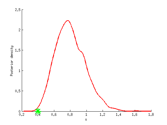
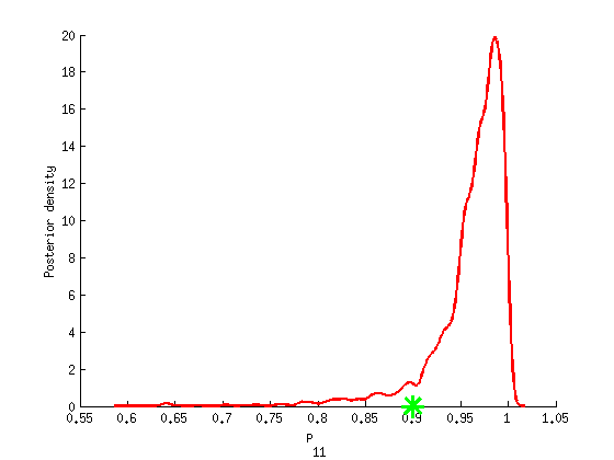
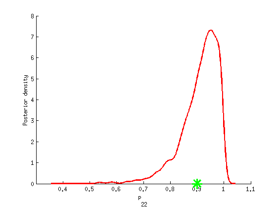
Histogram and KDE estimate of the posterior for the parameters
for k=1:numel(param_plot)
    figure('name', 'PMMH: Histogram posterior parameter')
    samples_param = getfield(out_pmmh, param_plot{k});
    hist(samples_param, 15)
    h = findobj(gca, 'Type', 'patch');
    set(h, 'EdgeColor', 'w', 'FaceColor', 'r')
    if sample_data
        hold on
        plot(param_true(k), 0, '*g', 'linewidth', 3, 'markersize', 16);
    end
    xlabel(param_lab{k}, 'fontsize', 24)
    ylabel('Number of samples', 'fontsize', 24)
    box off
%     title(param_lab{k})
    saveas(gca, ['switch_stoch_param', num2str(k)], 'epsc2')
    saveas(gca, ['switch_stoch_param', num2str(k)], 'png')
end

for k=1:numel(param_plot)
    figure('name', 'PMMH: KDE estimate posterior parameter')
    kde_param = getfield(kde_pmmh, param_plot{k});
    plot(kde_param.x, kde_param.f, 'r')
    if sample_data
        hold on
        plot(param_true(k), 0, '*g', 'linewidth', 3, 'markersize', 16);
    end
    xlabel(param_lab{k}, 'fontsize', 24)
    ylabel('Posterior density', 'fontsize', 24)
    box off
%     title(param_lab{k})
    saveas(gca, ['switch_stoch_param_kde', num2str(k)], 'epsc2')
    saveas(gca, ['switch_stoch_param_kde', num2str(k)], 'png')
end
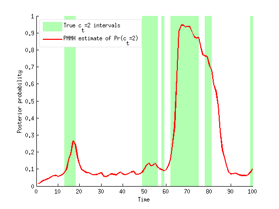
Posterior probability of c[t]=2
prob_c2 = zeros(1,t_max);
figure('name', 'PMMH: Posterior probabilities of c[t]=2')
hold on
for t=1:t_max
    if data.c_true(t)==2
        h = fill([t-1,t,t,t-1], [0,0,1,1], 0);
        set(h, 'edgecolor', 'none', 'facecolor', light_green)
        set(get(get(h,'Annotation'),'LegendInformation'),'IconDisplayStyle','off')
    end
    ind = find(table_c(t).x == 2);
    if isempty(ind)
        prob_c2(t) = 1-sum(table_c(t).f);
    else
        prob_c2(t) = table_c(t).f(ind);
    end
end
set(get(get(h,'Annotation'),'LegendInformation'),'IconDisplayStyle','on')
plot(1:t_max, prob_c2, 'r')
xlabel('Time')
ylabel('Posterior probability')
legend({'True c_t=2 intervals', 'PMMH estimate of Pr(c_t=2)'},...
    'Location', 'NorthWest', 'EdgeColor', light_gray)
saveas(gca, 'switch_stoch_param_c', 'epsc2')
saveas(gca, 'switch_stoch_param_c', 'png')
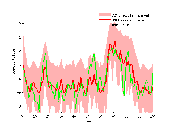
Posterior mean and quantiles for x
figure('name', 'PMMH: Posterior mean and quantiles')
x_pmmh_mean = summ_pmmh.x.mean;
x_pmmh_quant = summ_pmmh.x.quant;
h = fill([1:t_max, t_max:-1:1], [x_pmmh_quant{1}; flipud(x_pmmh_quant{2})], 0);
set(h, 'edgecolor', 'none', 'facecolor', light_red)
hold on
plot(1:t_max, x_pmmh_mean, 'r', 'linewidth', 3)
if sample_data
    plot(1:t_max, data.x_true, 'g')
    legend({'95% credible interval', 'PMMH mean estimate', 'True value'})
else
    legend({'95% credible interval', 'PMMH mean estimate'})
end
ylim([-6.5,1])
xlabel('Time')
ylabel('Log-volatility')
box off
legend boxoff
saveas(gca, 'switch_stoch_param_x', 'epsc2')
saveas(gca, 'switch_stoch_param_x', 'png')
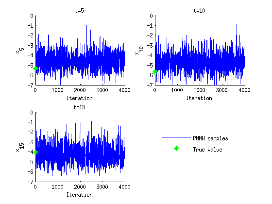
Trace of MCMC samples for x
figure('name', 'PMMH: Trace samples x')
time_index = [5, 10, 15];
for k=1:numel(time_index)
    tk = time_index(k);
    subplot(2, 2, k)
    plot(out_pmmh.x(tk, :), 'linewidth', 1)
    if sample_data
        hold on
        plot(0, data.x_true(tk), '*g');
    end
    ylim([-7,0])
    xlabel('Iteration')
    ylabel(['x_{', num2str(tk), '}'])
    title(['t=', num2str(tk)]);
    box off
end
if sample_data
    h = legend({'PMMH samples', 'True value'});
    set(h, 'position', [0.7, 0.25, .1, .1])
    legend boxoff
end
saveas(gca, 'switch_stoch_param_x_trace', 'epsc2')
saveas(gca, 'switch_stoch_param_x_trace', 'png')
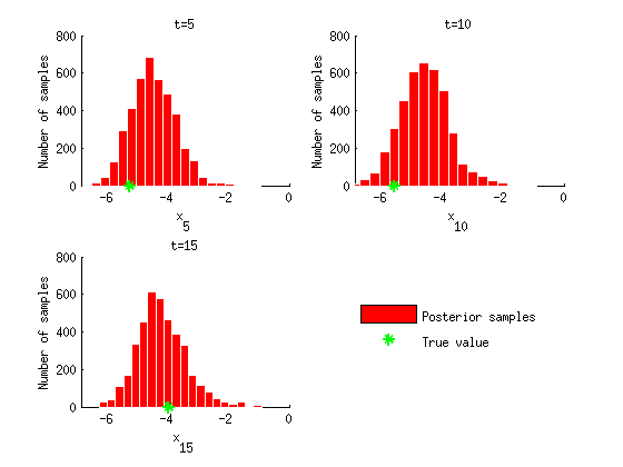
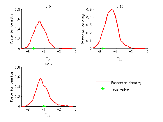
Histogram and kernel density estimate of posteriors of x
figure('name', 'PMMH: Histograms marginal posteriors')
for k=1:numel(time_index)
    tk = time_index(k);
    subplot(2, 2, k)
    hist(out_pmmh.x(tk, :), 20);
    h = findobj(gca, 'Type', 'patch');
    set(h, 'EdgeColor', 'w', 'FaceColor', 'r')
    if sample_data
        hold on
        plot(data.x_true(tk), 0, '*g');
    end
    xlim([-7,0])
    xlabel(['x_{', num2str(tk), '}']);
    ylabel('Number of samples');
    title(['t=', num2str(tk)]);
    box off
end
if sample_data
    h = legend({'Posterior samples', 'True value'});
    set(h, 'position', [0.7, 0.25, .1, .1])
    legend boxoff
end
saveas(gca, 'switch_stoch_param_x_hist', 'epsc2')
saveas(gca, 'switch_stoch_param_x_hist', 'png')

figure('name', 'PMMH: KDE estimates marginal posteriors')
for k=1:numel(time_index)
    tk = time_index(k);
    subplot(2, 2, k)
    plot(kde_pmmh.x(tk).x, kde_pmmh.x(tk).f, 'r');
    if sample_data
        hold on
        plot(data.x_true(tk), 0, '*g');
    end
    xlim([-7,0])
    xlabel(['x_{', num2str(tk), '}']);
    ylabel('Posterior density');
    title(['t=', num2str(tk)]);
    box off
end
if sample_data
    h = legend({'Posterior density', 'True value'});
    set(h, 'position', [0.7, 0.25, .1, .1])
    legend boxoff
end
saveas(gca, 'switch_stoch_param_x_kde', 'epsc2')
saveas(gca, 'switch_stoch_param_x_kde', 'png')
Clear model
biips_clear()

save switch_stoch_param_workspace.mat