Matbiips example: Switching stochastic volatility
In this example, we consider the Markov switching stochastic volatility model.
Reference: C.M. Carvalho and H.F. Lopes. Simulation-based sequential analysis of Markov switching stochastic volatility models. Computational Statistics and Data analysis (2007) 4526-4542.
Contents
Statistical model
Let  be the response variable and
  the unobserved log-volatility of . The stochastic volatility model is defined as follows for

The regime variables  follow a two-state Markov process with transition probabilities

 denotes the normal distribution of mean
  and variance
  .
.
Statistical model in BUGS language
Content of the file 'switch_stoch_volatility.bug':
model_file = 'switch_stoch_volatility.bug'; % BUGS model filename
type(model_file);
var y[t_max],x[t_max],mu[t_max],mu_true[t_max],c[t_max],c_true[t_max]
data
{
c_true[1] ~ dcat(pi[c0,])
mu_true[1] <- alpha[1] * (c_true[1]==1) + alpha[2]*(c_true[1]==2) + phi*x0
x_true[1] ~ dnorm(mu_true[1], 1/sigma^2)
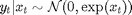
y[1] ~ dnorm(0, exp(-x_true[1]))
for (t in 2:t_max)
{
c_true[t] ~ dcat(ifelse(c_true[t-1]==1,pi[1,],pi[2,]))
mu_true[t] <- alpha[1]*(c_true[t]==1) + alpha[2]*(c_true[t]==2) + phi*x_true[t-1];
x_true[t] ~ dnorm(mu_true[t], 1/sigma^2)
y[t] ~ dnorm(0, exp(-x_true[t]))
}
}
model
{
c[1] ~ dcat(pi[c0,])
mu[1] <- alpha[1] * (c[1]==1) + alpha[2]*(c[1]==2)+ phi*x0
x[1] ~ dnorm(mu[1], 1/sigma^2)
y[1] ~ dnorm(0, exp(-x[1]))
for (t in 2:t_max)
{
c[t] ~ dcat(ifelse(c[t-1]==1, pi[1,], pi[2,]))
mu[t] <- alpha[1] * (c[t]==1) + alpha[2]*(c[t]==2) + phi*x[t-1]
x[t] ~ dnorm(mu[t], 1/sigma^2)
y[t] ~ dnorm(0, exp(-x[t]))
}
}
Installation of Matbiips
- Download the latest version of Matbiips
- Unzip the archive in some folder
- Add the Matbiips folder to the Matlab search path
matbiips_path = '../../matbiips';
addpath(matbiips_path)
General settings
set(0, 'DefaultAxesFontsize', 16);
set(0, 'Defaultlinelinewidth', 2);
set(0, 'DefaultLineMarkerSize', 8);
light_blue = [.7, .7, 1];
light_red = [1, .7, .7];

% Set the random numbers generator seed for reproducibility
if isoctave() || verLessThan('matlab', '7.12')
    rand('state', 0)
else
    rng('default')
end
Load model and data
Model parameters
t_max = 100;
sigma = .4; alpha = [-2.5; -1]; phi = .5; c0 = 1; x0 = 0;
pi = [.9, .1; .1, .9];
data = struct('t_max', t_max, 'sigma', sigma,...
    'alpha', alpha, 'phi', phi, 'pi', pi, 'c0', c0, 'x0', x0);
Parse and compile BUGS model, and sample data
model = biips_model(model_file, data, 'sample_data', true);
data = model.data;
* Parsing model in: switch_stoch_volatility.bug
* Compiling data graph
  Declaring variables
  Resolving undeclared variables
  Allocating nodes
  Graph size: 1215
  Sampling data
  Reading data back into data table
* Compiling model graph
  Declaring variables
  Resolving undeclared variables
  Allocating nodes
  Graph size: 1218
Plot the data
figure('name', 'Log-returns')
plot(1:t_max, data.y)
title('Observed data')
xlabel('Time')
ylabel('Log-return')
box off
saveas(gca, 'volatility_obs', 'epsc2')
saveas(gca, 'volatility_obs', 'png')
Biips Sequential Monte Carlo
Run SMC
n_part = 5000; % Number of particles
variables = {'x'}; % Variables to be monitored
out_smc = biips_smc_samples(model, variables, n_part);
* Assigning node samplers
* Running SMC forward sampler with 5000 particles
  |--------------------------------------------------| 100%
  |**************************************************| 100 iterations in 9.91 s
Diagnosis of the algorithm.
diag_smc = biips_diagnosis(out_smc);
* Diagnosis of variable: x[1:100]
  Filtering: GOOD
  Smoothing: GOOD
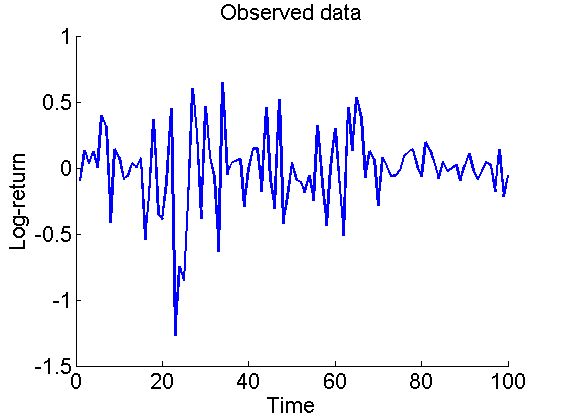
Plot Smoothing ESS
figure('name', 'SMC: SESS')
semilogy(1:t_max, out_smc.x.s.ess)
hold on
plot(1:t_max, 30*ones(t_max,1), '--k')
xlabel('Time')
ylabel('SESS')
box off
saveas(gca, 'volatility_ess', 'epsc2')
saveas(gca, 'volatility_ess', 'png')
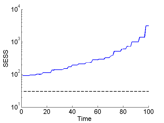
Plot weighted particles
figure('name', 'SMC: Particles (smoothing)')
hold on
for t=1:t_max
    val = unique(out_smc.x.s.values(t,:));

    weight = arrayfun(@(x) sum(out_smc.x.s.weights(t, out_smc.x.s.values(t,:) == x)), val);

    scatter(t*ones(size(val)), val, min(50, .5*n_part*weight), 'r',...
        'markerfacecolor', 'r')
end
xlabel('Time')
ylabel('Log-volatility')
saveas(gca, 'volatility_particles_s', 'epsc2')
saveas(gca, 'volatility_particles_s', 'png')
Summary statistics
summ_smc = biips_summary(out_smc, 'probs', [.025, .975]);
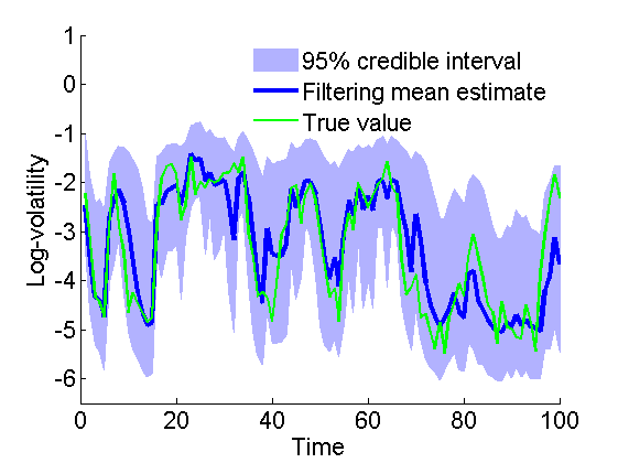
Plot Filtering estimates
figure('name', 'SMC: Filtering estimates')
x_f_mean = summ_smc.x.f.mean;
x_f_quant = summ_smc.x.f.quant;
h = fill([1:t_max, t_max:-1:1], [x_f_quant{1}; flipud(x_f_quant{2})], 0);
set(h, 'edgecolor', 'none', 'facecolor', light_blue)
hold on
plot(1:t_max, x_f_mean, 'linewidth', 3)
plot(1:t_max, data.x_true, 'g')
ylim([-6.5, 1])
xlabel('Time')
ylabel('Log-volatility')
legend({'95% credible interval', 'Filtering mean estimate', 'True value'})
legend boxoff
box off
saveas(gca, 'volatility_f', 'epsc2')
saveas(gca, 'volatility_f', 'png')
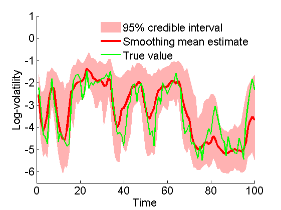
Plot Smoothing estimates
figure('name', 'SMC: Smoothing estimates')
x_s_mean = summ_smc.x.s.mean;
x_s_quant = summ_smc.x.s.quant;
h = fill([1:t_max, t_max:-1:1], [x_s_quant{1}; flipud(x_s_quant{2})], 0);
set(h, 'edgecolor', 'none', 'facecolor', light_red)
hold on
plot(1:t_max, x_s_mean, 'r', 'linewidth', 3)
plot(1:t_max, data.x_true, 'g')
ylim([-6.5, 1])
xlabel('Time')
ylabel('Log-volatility')
legend({'95% credible interval', 'Smoothing mean estimate', 'True value'})
legend boxoff
box off
saveas(gca, 'volatility_s', 'epsc2')
saveas(gca, 'volatility_s', 'png')
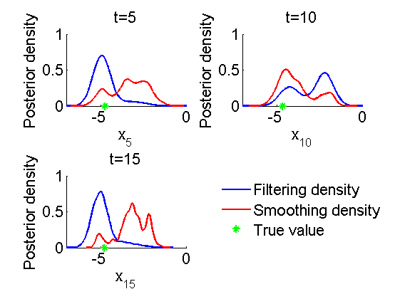
Marginal filtering and smoothing densities
figure('name', 'SMC: Marginal posteriors')
kde_smc = biips_density(out_smc);
time_index = [5, 10, 15];
for k=1:numel(time_index)
    tk = time_index(k);
    subplot(2, 2, k)
    plot(kde_smc.x.f(tk).x, kde_smc.x.f(tk).f);
    hold on
    plot(kde_smc.x.s(tk).x, kde_smc.x.s(tk).f, 'r');
    plot(data.x_true(tk), 0, '*g');
    xlim([-7,0])
    xlabel(['x_{', num2str(tk), '}']);
    ylabel('Posterior density');
    title(['t=', num2str(tk)]);
    box off
end
h =legend({'Filtering density', 'Smoothing density', 'True value'});
set(h, 'position',[0.7, 0.25, .1, .1])
legend boxoff
saveas(gca, 'volatility_kde', 'epsc2')
saveas(gca, 'volatility_kde', 'png')
Biips Particle Independent Metropolis-Hastings
Parameters of the PIMH
n_burn = 2000;
n_iter = 10000;
thin = 1;
n_part = 50;
Run PIMH
obj_pimh = biips_pimh_init(model, variables);
obj_pimh = biips_pimh_update(obj_pimh, n_burn, n_part); % burn-in iterations
[obj_pimh, out_pimh, log_marg_like_pimh] = biips_pimh_samples(obj_pimh,...
    n_iter, n_part, 'thin', thin);
* Initializing PIMH
* Updating PIMH with 50 particles
  |--------------------------------------------------| 100%
  |**************************************************| 2000 iterations in 139.74 s
* Generating PIMH samples with 50 particles
  |--------------------------------------------------| 100%
  |**************************************************| 10000 iterations in 733.44 s
Some summary statistics
summ_pimh = biips_summary(out_pimh, 'probs', [.025, .975]);
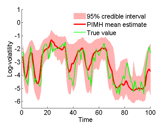
Posterior mean and quantiles
figure('name', 'PIMH: Posterior mean and quantiles')
x_pimh_mean = summ_pimh.x.mean;
x_pimh_quant = summ_pimh.x.quant;
h = fill([1:t_max, t_max:-1:1], [x_pimh_quant{1}; flipud(x_pimh_quant{2})], 0);
set(h, 'edgecolor', 'none', 'facecolor', light_red)
hold on
plot(1:t_max, x_pimh_mean, 'r', 'linewidth', 3)
plot(1:t_max, data.x_true, 'g')
ylim([-6.5, 1])
xlabel('Time')
ylabel('Log-volatility')
legend({'95% credible interval', 'PIMH mean estimate', 'True value'})
legend boxoff
box off
saveas(gca, 'volatility_pimh_s', 'epsc2')
saveas(gca, 'volatility_pimh_s', 'png')
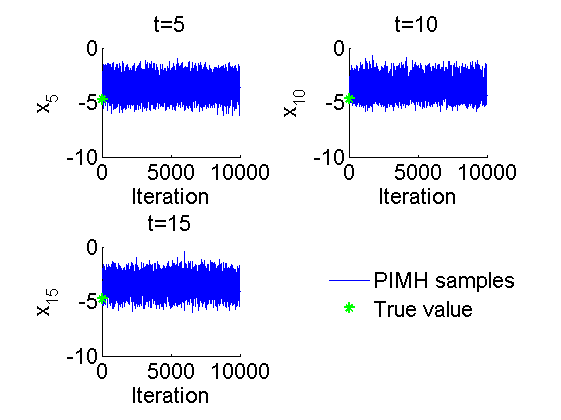
Trace of MCMC samples
figure('name', 'PIMH: Trace samples')
time_index = [5, 10, 15];
for k=1:numel(time_index)
    tk = time_index(k);
    subplot(2, 2, k)
    plot(out_pimh.x(tk, :), 'linewidth', 1)
    hold on
    plot(0, data.x_true(tk), '*g');
    xlabel('Iteration')
    ylabel(['x_{', num2str(tk), '}'])
    title(['t=', num2str(tk)]);
    box off
end
h = legend({'PIMH samples', 'True value'});
set(h, 'position', [0.7, 0.25, .1, .1])
legend boxoff
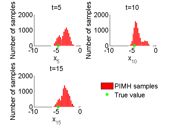
Histograms of posteriors
figure('name', 'PIMH: Histograms marginal posteriors')
for k=1:numel(time_index)
    tk = time_index(k);
    subplot(2, 2, k)
    hist(out_pimh.x(tk, :), 20);
    h = findobj(gca, 'Type', 'patch');
    set(h, 'EdgeColor', 'w', 'FaceColor', 'r')
    hold on
    plot(data.x_true(tk), 0, '*g');
    xlabel(['x_{', num2str(tk), '}']);
    ylabel('Number of samples');
    title(['t=', num2str(tk)]);
    box off
end
h =legend({'PIMH samples', 'True value'});
set(h, 'position', [0.7, 0.25, .1, .1])
legend boxoff
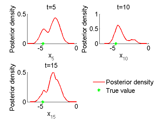
Kernel density estimates of posteriors
figure('name', 'PIMH: KDE estimates marginal posteriors')
kde_pimh = biips_density(out_pimh);
for k=1:numel(time_index)
    tk = time_index(k);
    subplot(2, 2, k)
    plot(kde_pimh.x(tk).x, kde_pimh.x(tk).f, 'r');
    hold on
    plot(data.x_true(tk), 0, '*g');
    xlim([-7,0])
    xlabel(['x_{', num2str(tk), '}']);
    ylabel('Posterior density');
    title(['t=', num2str(tk)]);
    box off
end
h = legend({'Posterior density', 'True value'});
set(h, 'position', [0.7, 0.25, .1, .1])
legend boxoff
saveas(gca, 'volatility_pimh_kde', 'epsc2')
saveas(gca, 'volatility_pimh_kde', 'png')
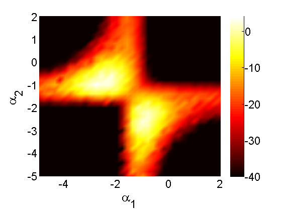
Biips Sensitivity analysis
We want to study sensitivity to the values of the parameter 
Parameters of the algorithm
n_part = 50; % Number of particles
param_names = {'alpha'}; % Parameter for which we want to study sensitivity
range = -5:.2:2; % Range of values for one component
[A, B] = meshgrid(range, range); % Grid of values for two components
param_values = {[A(:), B(:)]'};
Run sensitivity analysis with SMC
out_sens = biips_smc_sensitivity(model, param_names, param_values, n_part);
* Analyzing sensitivity with 50 particles
  |--------------------------------------------------| 100%
  |**************************************************| 1296 iterations in 87.20 s
Plot log-marginal likelihood and penalized log-marginal likelihood
figure('name', 'Sensitivity: Log-likelihood')
surf(A, B, reshape(out_sens.log_marg_like, size(A)))
view(2); colormap(hot); shading interp
caxis([-40, max(out_sens.log_marg_like(:))])
colorbar box off
box off
xlim([-5, 2])
xlabel('\alpha_1', 'fontsize', 20)
ylabel('\alpha_2', 'fontsize', 20)
saveas(gca, 'volatility_sensitivity', 'epsc2')
saveas(gca, 'volatility_sensitivity', 'png')
Clear model
biips_clear()