Matbiips example: Stochastic volatility
In this example, we consider the stochastic volatility model SV0 for application e.g. in finance.
Reference: S. Chib, F. Nardari, N. Shepard. Markov chain Monte Carlo methods for stochastic volatility models. Journal of econometrics, vol. 108, pp. 281-316, 2002.
Contents
Statistical model
The stochastic volatility model is defined as follows

and for 

where  is the response variable and
  is the unobserved log-volatility of .
  denotes the normal distribution of mean
  and variance
  .
.
 ,
,  and
and  are unknown parameters that need to be estimated.
Statistical model in BUGS language
Content of the file 'stoch_volatility.bug':
model_file = 'stoch_volatility.bug'; % BUGS model filename
type(model_file);
# Stochastic volatility model SV_0
# Reference: S. Chib, F. Nardari, N. Shepard. Markov chain Monte Carlo methods
# for stochastic volatility models. Journal of econometrics, vol. 108, pp. 281-316, 2002.

var y[t_max], x[t_max], prec_y[t_max]

data
{
  x_true[1] ~ dnorm(0, 1/sigma_true^2)
  prec_y_true[1] <- exp(-x_true[1])
  y[1] ~ dnorm(0, prec_y_true[1])
  for (t in 2:t_max)
  {
    x_true[t] ~ dnorm(alpha_true + beta_true*(x_true[t-1]-alpha_true), 1/sigma_true^2)
    prec_y_true[t] <- exp(-x_true[t])
    y[t] ~ dnorm(0, prec_y_true[t])
  }
}

model
{
  alpha ~ dnorm(0,10000)
  logit_beta ~ dnorm(0,.1)
  beta <- ilogit(logit_beta)
  log_sigma ~ dnorm(0, 1)
  sigma <- exp(log_sigma)

  x[1] ~ dnorm(0, 1/sigma^2)
  prec_y[1] <- exp(-x[1])
  y[1] ~ dnorm(0, prec_y[1])
  for (t in 2:t_max)
  {
    x[t] ~ dnorm(alpha + beta*(x[t-1]-alpha), 1/sigma^2)
    prec_y[t] <- exp(-x[t])
    y[t] ~ dnorm(0, prec_y[t])
  }
}
Installation of Matbiips
- Download the latest version of Matbiips
- Unzip the archive in some folder
- Add the Matbiips folder to the Matlab search path
matbiips_path = '../../matbiips';
addpath(matbiips_path)
General settings
set(0, 'DefaultAxesFontsize', 14);
set(0, 'Defaultlinelinewidth', 2);
light_blue = [.7, .7, 1];

% Set the random numbers generator seed for reproducibility
if isoctave() || verLessThan('matlab', '7.12')
    rand('state', 0)
else
    rng('default')
end
Load model and load or simulate data
sample_data = true; % Simulated data or SP500 data
t_max = 100;

if ~sample_data
    % Load the data
    T = readtable('SP500.csv', 'delimiter', ';');
    y = diff(log(T.Close(end:-1:1)));
    SP500_date_str = T.Date(end:-1:2);

    ind = 1:t_max;
    y = y(ind);
    SP500_date_str = SP500_date_str(ind);

    SP500_date_num = datenum(SP500_date_str);
end
Model parameters
if ~sample_data
    data = struct('t_max', t_max, 'y', y);
else
    sigma_true = .4;
    alpha_true = 0;
    beta_true = .99;
    data = struct('t_max', t_max, 'sigma_true', sigma_true,...
        'alpha_true', alpha_true, 'beta_true', beta_true);
end
Compile BUGS model and sample data if simulated data
model = biips_model(model_file, data, 'sample_data', sample_data);
data = model.data;
* Parsing model in: stoch_volatility.bug
* Compiling data graph
  Declaring variables
  Resolving undeclared variables
  Allocating nodes
  Graph size: 706
  Sampling data
  Reading data back into data table
* Compiling model graph
  Declaring variables
  Resolving undeclared variables
  Allocating nodes
  Graph size: 715
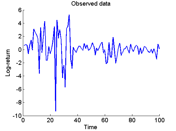
Plot the data
figure('name', 'Log-returns')
if sample_data
    plot(1:t_max, data.y)
    title('Observed data')
    xlabel('Time')
else
    plot(SP500_date_num, data.y)
    title('Observed data: S&P 500')
    datetick('x', 'mmmyyyy', 'keepticks')
    xlabel('Date')
end
ylabel('Log-return')
box off
Biips Particle Marginal Metropolis-Hastings
We now use Biips to run a Particle Marginal Metropolis-Hastings in order to obtain posterior MCMC samples of the parameters , and , and of the variables  .
.
Parameters of the PMMH
n_burn = 5000; % nb of burn-in/adaptation iterations
n_iter = 10000; % nb of iterations after burn-in
thin = 5; % thinning of MCMC outputs
n_part = 50; % nb of particles for the SMC

param_names = {'alpha', 'logit_beta', 'log_sigma'}; % names of the variables updated with MCMC (others are updated with SMC)
latent_names = {'x'}; % names of the variables updated with SMC and that need to be monitored
Init PMMH
inits = {0, 5, -2};
obj_pmmh = biips_pmmh_init(model, param_names, 'inits', inits,...
    'latent_names', latent_names);
* Initializing PMMH
Run PMMH
obj_pmmh = biips_pmmh_update(obj_pmmh, n_burn, n_part); % adaptation and burn-in iterations
[obj_pmmh, out_pmmh, log_marg_like_pen, log_marg_like] = biips_pmmh_samples(obj_pmmh, n_iter, n_part,...
    'thin', thin); % Samples
* Adapting PMMH with 50 particles
  |--------------------------------------------------| 100%
  |++++++++++++++++++++++++++++++++++++++++++++++++++| 5000 iterations in 203.25 s
* Generating 2000 PMMH samples with 50 particles
  |--------------------------------------------------| 100%
  |**************************************************| 10000 iterations in 381.09 s
Some summary statistics
summ_pmmh = biips_summary(out_pmmh, 'probs', [.025, .975]);
Compute kernel density estimates
kde_pmmh = biips_density(out_pmmh);
Posterior mean and credible interval of the parameters
for i=1:numel(param_names)
    summ_param = getfield(summ_pmmh, param_names{i});
    fprintf('Posterior mean of %s: %.3f\n', param_names{i}, summ_param.mean);
    fprintf('95%% credible interval of %s: [%.3f, %.3f]\n',...
        param_names{i}, summ_param.quant{1}, summ_param.quant{2});
end
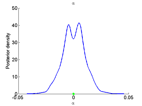
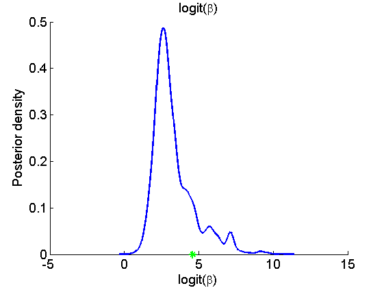
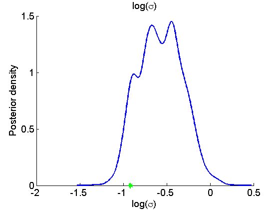
Posterior mean of alpha: 0.000
95% credible interval of alpha: [-0.020, 0.020]
Posterior mean of logit_beta: 3.309
95% credible interval of logit_beta: [1.521, 7.178]
Posterior mean of log_sigma: -0.571
95% credible interval of log_sigma: [-1.009, -0.110]
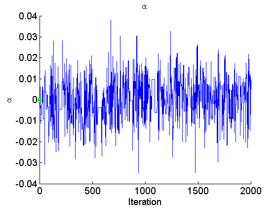
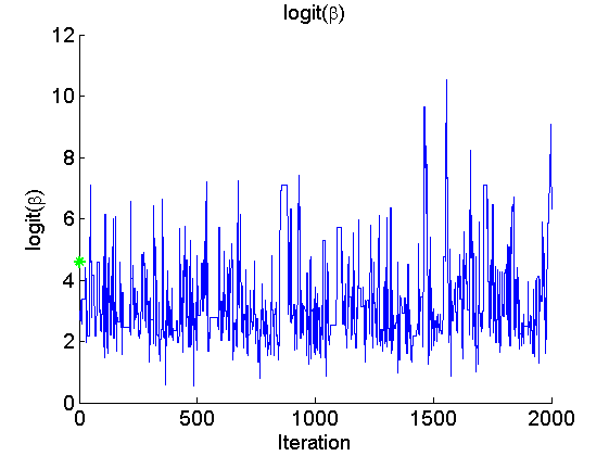
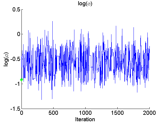
Trace of MCMC samples for the parameters
if sample_data
    param_true = [alpha_true, log(data.beta_true/(1-data.beta_true)), log(sigma_true)];
end
param_lab = {'\alpha', 'logit(\beta)', 'log(\sigma)'};

for k=1:numel(param_names)
    figure('name', 'PMMH: Trace samples parameter')
    samples_param = getfield(out_pmmh, param_names{k});
    plot(samples_param, 'linewidth', 1)
    if sample_data
        hold on
        plot(0, param_true(k), '*g');
    end
    xlabel('Iteration')
    ylabel(param_lab{k})
    title(param_lab{k})
    box off
    legend boxoff
end
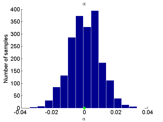
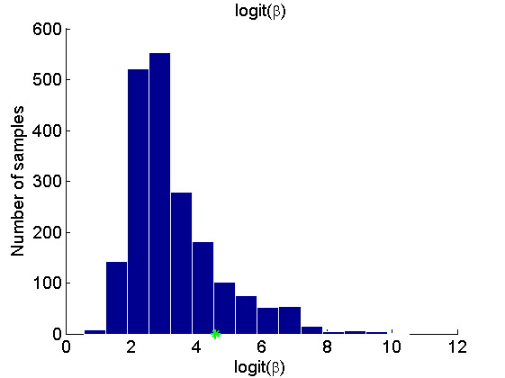
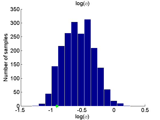
Histogram and KDE estimate of the posterior for the parameters
for k=1:numel(param_names)
    figure('name', 'PMMH: Histogram posterior parameter')
    samples_param = getfield(out_pmmh, param_names{k});
    hist(samples_param, 15)
    h = findobj(gca, 'Type', 'patch');
    set(h, 'EdgeColor', 'w')
    if sample_data
        hold on
        plot(param_true(k), 0, '*g');
    end
    xlabel(param_lab{k})
    ylabel('Number of samples')
    title(param_lab{k})
    box off
    legend boxoff
end

for k=1:numel(param_names)
    figure('name', 'PMMH: KDE estimate posterior parameter')
    kde_param = getfield(kde_pmmh, param_names{k});
    plot(kde_param.x, kde_param.f)
    if sample_data
        hold on
        plot(param_true(k), 0, '*g');
    end
    xlabel(param_lab{k})
    ylabel('Posterior density')
    title(param_lab{k})
    box off
    legend boxoff
end
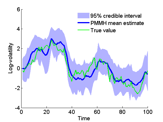
Posterior mean and quantiles for x
figure('name', 'PMMH: Posterior mean and quantiles')
x_pmmh_mean = summ_pmmh.x.mean;
x_pmmh_quant = summ_pmmh.x.quant;
h = fill([1:t_max, t_max:-1:1], [x_pmmh_quant{1}; flipud(x_pmmh_quant{2})], 0);
set(h, 'edgecolor', 'none', 'facecolor', light_blue)
hold on
plot(1:t_max, x_pmmh_mean, 'linewidth', 3)
if sample_data
    plot(1:t_max, data.x_true, 'g')
    legend({'95% credible interval', 'PMMH mean estimate', 'True value'})
else
    legend({'95% credible interval', 'PMMH mean estimate'})
end
xlabel('Time')
ylabel('Log-volatility')
box off
legend boxoff
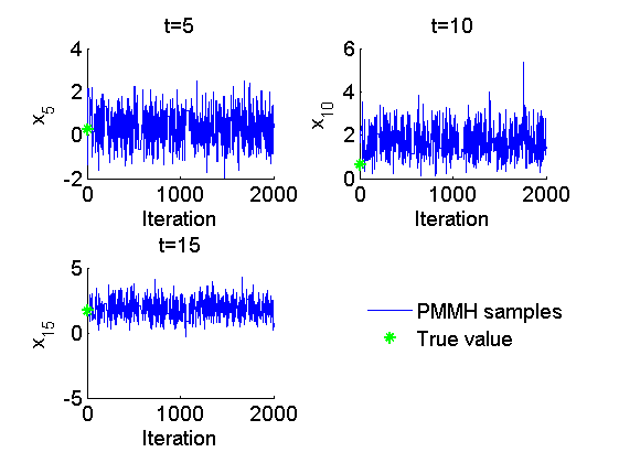
Trace of MCMC samples for x
figure('name', 'PMMH: Trace samples x')
time_index = [5, 10, 15];
for k=1:numel(time_index)
    tk = time_index(k);
    subplot(2, 2, k)
    plot(out_pmmh.x(tk, :), 'linewidth', 1)
    if sample_data
        hold on
        plot(0, data.x_true(tk), '*g');
    end
    xlabel('Iteration')
    ylabel(['x_{', num2str(tk), '}'])
    title(['t=', num2str(tk)]);
    box off
end
if sample_data
    h = legend({'PMMH samples', 'True value'});
    set(h, 'position', [0.7, 0.25, .1, .1])
    legend boxoff
end
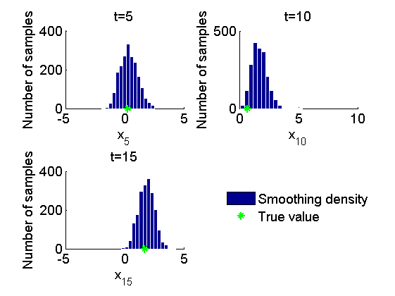
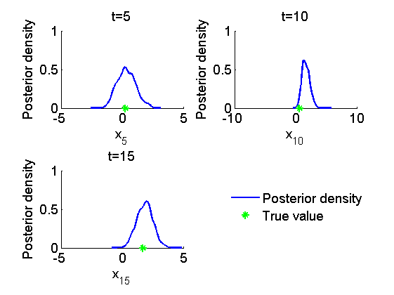
Histogram and kernel density estimate of posteriors of x
figure('name', 'PMMH: Histograms marginal posteriors')
for k=1:numel(time_index)
    tk = time_index(k);
    subplot(2, 2, k)
    hist(out_pmmh.x(tk, :), 15);
    h = findobj(gca, 'Type', 'patch');
    set(h, 'EdgeColor', 'w')
    if sample_data
        hold on
        plot(data.x_true(tk), 0, '*g');
    end
    xlabel(['x_{', num2str(tk), '}']);
    ylabel('Number of samples');
    title(['t=', num2str(tk)]);
    box off
end
if sample_data
    h = legend({'Smoothing density', 'True value'});
    set(h, 'position', [0.7, 0.25, .1, .1])
    legend boxoff
end

figure('name', 'PMMH: KDE estimates marginal posteriors')
for k=1:numel(time_index)
    tk = time_index(k);
    subplot(2, 2, k)
    plot(kde_pmmh.x(tk).x, kde_pmmh.x(tk).f);
    if sample_data
        hold on
        plot(data.x_true(tk), 0, '*g');
    end
    xlabel(['x_{', num2str(tk), '}']);
    ylabel('Posterior density');
    title(['t=', num2str(tk)]);
    box off
end
if sample_data
    h = legend({'Posterior density', 'True value'});
    set(h, 'position', [0.7, 0.25, .1, .1])
    legend boxoff
end
Clear model
biips_clear()