Matbiips example: Stochastic kinetic predator-prey model
Reference: A. Golightly and D. J. Wilkinson. Bayesian parameter inference for stochastic biochemical network models using particle Markov chain Monte Carlo. Interface Focus, vol.1, pp. 807-820, 2011.
Contents
Statistical model
Let  where
where  is an integer, and
  a multiple of . For

where 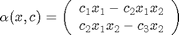 and
and 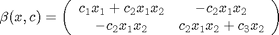
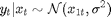
For  ,
, 
and for 
 and
and  respectively correspond to the number of preys and predators and
  is the approximated number of preys. The model is the approximation of the Lotka-Volterra model.
Statistical model in BUGS language
model_filename = 'stoch_kinetic_cle.bug'; % BUGS model filename
type(model_filename);
# Stochastic kinetic predator-prey model
# with chemical Langevin equations
#
# Reference: A. Golightly and D. J. Wilkinson. Bayesian parameter inference
# for stochastic biochemical network models using particle Markov chain
# Monte Carlo. Interface Focus, vol.1, pp. 807-820, 2011.
var x_true[2,t_max/dt], x_true_temp[2,t_max/dt],
x[2,t_max/dt], x_temp[2,t_max/dt], y[t_max/dt],
beta[2,2,t_max/dt], beta_true[2,2,t_max/dt],
logc[3], c[3], c_true[3]
data
{
x_true[,1] ~ dmnormvar(x_init_mean, x_init_var)
for (t in 2:t_max/dt)
{
alpha_true[1,t] <- c_true[1]*x_true[1,t-1] - c_true[2]*x_true[1,t-1]*x_true[2,t-1]
alpha_true[2,t] <- c_true[2]*x_true[1,t-1]*x_true[2,t-1] - c_true[3]*x_true[2,t-1]
beta_true[1,1,t] <- c_true[1]*x_true[1,t-1] + c_true[2]*x_true[1,t-1]*x_true[2,t-1]
beta_true[1,2,t] <- -c_true[2]*x_true[1,t-1]*x_true[2,t-1]
beta_true[2,1,t] <- beta_true[1,2,t]
beta_true[2,2,t] <- c_true[2]*x_true[1,t-1]*x_true[2,t-1] + c_true[3]*x_true[2,t-1]
x_true_temp[,t] ~ dmnormvar(x_true[,t-1]+alpha_true[,t]*dt, (beta_true[,,t])*dt)
# To avoid extinction
x_true[1,t] <- max(x_true_temp[1,t],1)
x_true[2,t] <- max(x_true_temp[2,t],1)
}
for (t in 1:t_max)
{
y[t/dt] ~ dnorm(x_true[1,t/dt], prec_y)
}
}
model
{
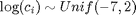
logc[1] ~ dunif(-7,2)
logc[2] ~ dunif(-7,2)
logc[3] ~ dunif(-7,2)
c[1] <- exp(logc[1])
c[2] <- exp(logc[2])
c[3] <- exp(logc[3])
x[,1] ~ dmnormvar(x_init_mean, x_init_var)
for (t in 2:t_max/dt)
{
alpha[1,t] <- c[1]*x[1,t-1] - c[2]*x[1,t-1]*x[2,t-1]
alpha[2,t] <- c[2]*x[1,t-1]*x[2,t-1] - c[3]*x[2,t-1]
beta[1,1,t] <- c[1]*x[1,t-1] + c[2]*x[1,t-1]*x[2,t-1]
beta[1,2,t] <- -c[2]*x[1,t-1]*x[2,t-1]
beta[2,1,t] <- beta[1,2,t]
beta[2,2,t] <- c[2]*x[1,t-1]*x[2,t-1] + c[3]*x[2,t-1]
x_temp[,t] ~ dmnormvar(x[,t-1]+alpha[,t]*dt, beta[,,t]*dt)
# To avoid extinction
x[1,t] <- max(x_temp[1,t],1)
x[2,t] <- max(x_temp[2,t],1)
}
for (t in 1:t_max)
{
y[t/dt] ~ dnorm(x[1,t/dt], prec_y)
}
}
Installation of Matbiips
- Download the latest version of Matbiips
- Unzip the archive in some folder
- Add the Matbiips folder to the Matlab search path
matbiips_path = '../../matbiips';
addpath(matbiips_path)
General settings
set(0, 'DefaultAxesFontsize', 14);
set(0, 'Defaultlinelinewidth', 2);
light_blue = [.7, .7, 1];
light_red = [1, .7, .7];
dark_blue = [0, 0, .5];
dark_red = [.5, 0, 0];

% Set the random numbers generator seed for reproducibility
if isoctave() || verLessThan('matlab', '7.12')
    rand('state', 0)
else
    rng('default')
end
Load model and data
Model parameters
t_max = 20;
dt = .2;
x_init_mean = [100; 100];
x_init_var = 10*eye(2);
c_true = [.5, .0025, .3];
prec_y = 1/10;
data = struct('t_max', t_max, 'dt', dt, 'c_true', c_true,...
    'x_init_mean', x_init_mean, 'x_init_var', x_init_var, 'prec_y', prec_y);
Compile BUGS model and sample data
sample_data = true; % Boolean
model = biips_model(model_filename, data, 'sample_data', sample_data); % Create Biips model and sample data
data = model.data;
* Parsing model in: stoch_kinetic_cle.bug
* Compiling data graph
  Declaring variables
  Resolving undeclared variables
  Allocating nodes
  Graph size: 1914
  Sampling data
  Reading data back into data table
* Compiling model graph
  Declaring variables
  Resolving undeclared variables
  Allocating nodes
  Graph size: 2713
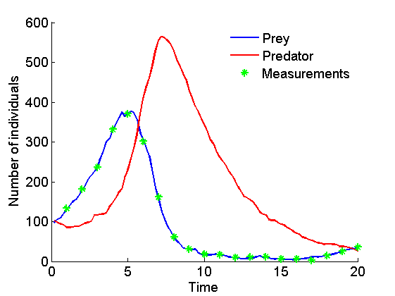
Plot data
figure('name', 'Data')
t_vec = dt:dt:t_max;
plot(t_vec, data.x_true(1,:))
hold on
plot(t_vec, data.x_true(2,:), 'r')
plot(t_vec, data.y, 'g*')
xlabel('Time')
ylabel('Number of individuals')
legend('Prey', 'Predator', 'Measurements')
box off
legend boxoff
Biips Sensitivity analysis with Sequential Monte Carlo
Parameters of the algorithm
n_part = 100; % Number of particles
param_names = {'logc[1]', 'logc[2]', 'logc[3]'}; % Parameter for which we want to study sensitivity
n_grid = 20;
param_values = {linspace(-7,1,n_grid), repmat(log(c_true(2)), n_grid, 1), repmat(log(c_true(3)), n_grid, 1)}; % Range of values

% n_grid = 5;
% [param_values{1:3}] = meshgrid(linspace(-7,1,n_grid), linspace(-7,1,n_grid), linspace(-7,1,n_grid));
% param_values = cellfun(@(x) x(:), param_values, 'uniformoutput', false);
Run sensitivity analysis with SMC
out_sens = biips_smc_sensitivity(model, param_names, param_values, n_part);
* Analyzing sensitivity with 100 particles
  |--------------------------------------------------| 100%
  |**************************************************| 20 iterations in 3.88 s
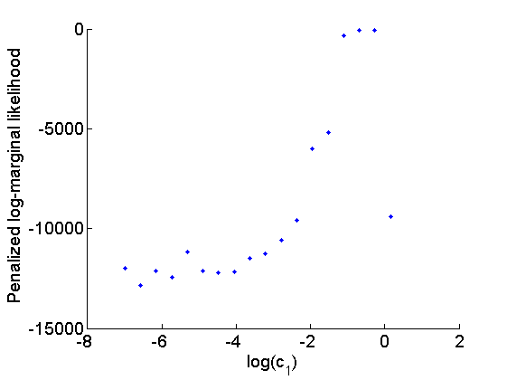
Plot penalized log-marginal likelihood
figure('name', 'Sensitivity: Penalized log-marginal likelihood');
plot(param_values{1}, out_sens.log_marg_like_pen, '.')
xlabel('log(c_1)')
ylabel('Penalized log-marginal likelihood')
ylim([-15000, 0])
box off
Biips Particle Marginal Metropolis-Hastings
We now use Biips to run a Particle Marginal Metropolis-Hastings in order to obtain posterior MCMC samples of the parameters and variables  .
.
Parameters of the PMMH
n_burn = 2000; % nb of burn-in/adaptation iterations
n_iter = 20000; % nb of iterations after burn-in
thin = 10; % thinning of MCMC outputs
n_part = 100; % nb of particles for the SMC

param_names = {'logc[1]', 'logc[2]', 'logc[3]'}; % names of the variables updated with MCMC (others are updated with SMC)
latent_names = {'x'}; % names of the variables updated with SMC and that need to be monitored
Init PMMH
obj_pmmh = biips_pmmh_init(model, param_names, 'inits', {-1, -5, -1},...
    'latent_names', latent_names); % creates a pmmh object
* Initializing PMMH
Run PMMH
obj_pmmh = biips_pmmh_update(obj_pmmh, n_burn, n_part); % adaptation and burn-in iterations
[obj_pmmh, out_pmmh, log_marg_like_pen] = biips_pmmh_samples(obj_pmmh, n_iter, n_part,...
    'thin', thin); % Samples
* Adapting PMMH with 100 particles
  |--------------------------------------------------| 100%
  |++++++++++++++++++++++++++++++++++++++++++++++++++| 2000 iterations in 293.14 s
* Generating 2000 PMMH samples with 100 particles
  |--------------------------------------------------| 100%
  |**************************************************| 20000 iterations in 3455.99 s
Some summary statistics
summ_pmmh = biips_summary(out_pmmh, 'probs', [.025, .975]);
Compute kernel density estimates
kde_pmmh = biips_density(out_pmmh);
param_true = log(c_true);
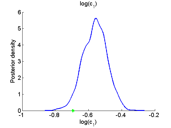
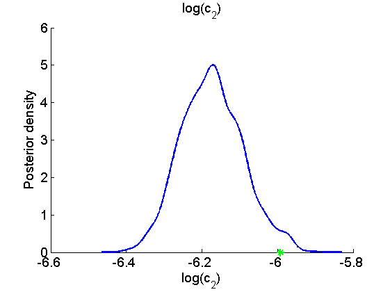
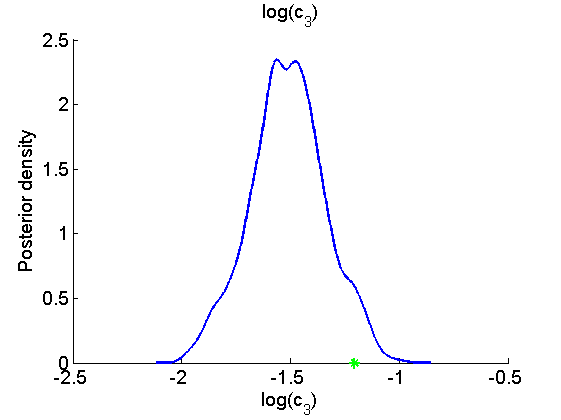
param_lab = {'log(c_1)', 'log(c_2)', 'log(c_3)'};
Posterior mean and credible interval of the parameters
for i=1:numel(param_names)
    summ_param = getfield(summ_pmmh, param_names{i});
    fprintf('Posterior mean of %s: %.3f\n', param_names{i}, summ_param.mean);
    fprintf('95%% credibile interval of %s: [%.1f, %.1f]\n',...
        param_names{i}, summ_param.quant{1}, summ_param.quant{2});
end
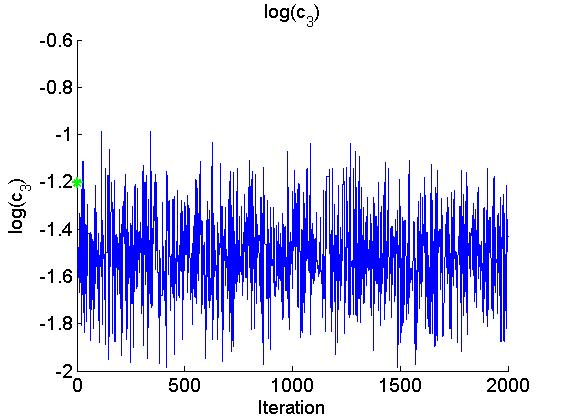
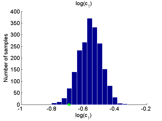
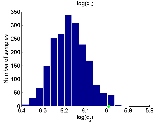
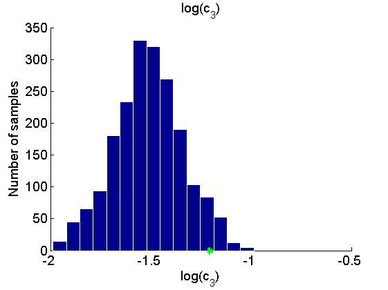
Posterior mean of logc[1]: -0.561
95% credibile interval of logc[1]: [-0.7, -0.4]
Posterior mean of logc[2]: -6.174
95% credibile interval of logc[2]: [-6.3, -6.0]
Posterior mean of logc[3]: -1.512
95% credibile interval of logc[3]: [-1.9, -1.2]
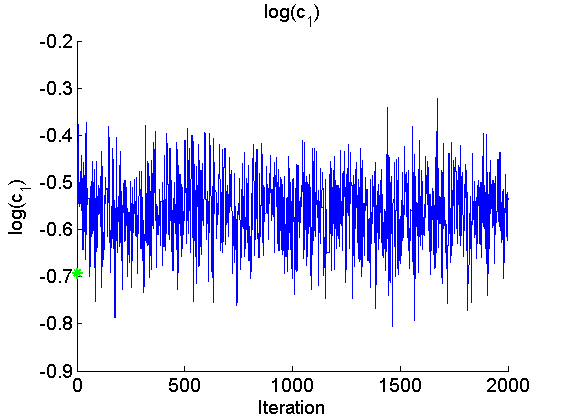
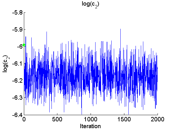
Trace of MCMC samples for the parameters
for i=1:numel(param_names)
    figure('name', 'PMMH: Trace samples parameter')
    samples_param = getfield(out_pmmh, param_names{i});
    plot(samples_param, 'linewidth', 1);
    hold on
    plot(0, param_true(i), '*g');
    xlabel('Iteration')
    ylabel(param_lab{i})
    title(param_lab{i})
    box off
end
Histogram and KDE estimate of the posterior for the parameters
for i=1:numel(param_names)
    figure('name', 'PMMH: Histogram posterior parameter')
    samples_param = getfield(out_pmmh, param_names{i});
    hist(samples_param, 15)
    h = findobj(gca, 'Type', 'patch');
    set(h, 'EdgeColor', 'w')
    hold on
    plot(param_true(i), 0, '*g');
    xlabel(param_lab{i})
    ylabel('Number of samples')
    title(param_lab{i})
    box off
end

for i=1:numel(param_names)
    figure('name', 'PMMH: KDE estimate posterior parameter')
    kde_param = getfield(kde_pmmh, param_names{i});
    plot(kde_param.x, kde_param.f);
    hold on
    plot(param_true(i), 0, '*g');
    xlabel(param_lab{i});
    ylabel('Posterior density');
    title(param_lab{i})
    box off
end
Posterior mean and quantiles for x
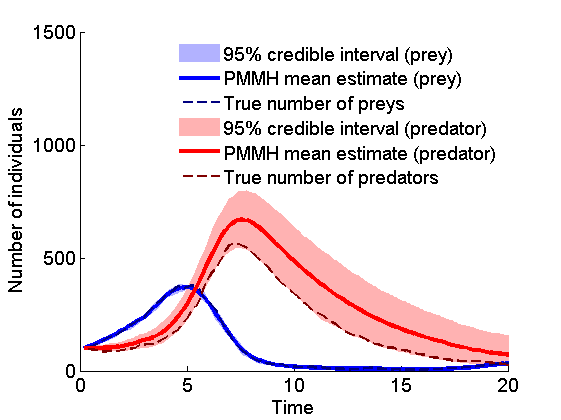
figure('name', 'PMMH: Posterior mean and quantiles')
x_pmmh_mean = summ_pmmh.x.mean;
x_pmmh_quant = summ_pmmh.x.quant;
h = fill([t_vec, fliplr(t_vec)], [x_pmmh_quant{1}(1,:), fliplr(x_pmmh_quant{2}(1,:))], 0);
set(h, 'edgecolor', 'none', 'facecolor', light_blue)
hold on
plot(t_vec, x_pmmh_mean(1, :), 'linewidth', 3)
plot(t_vec, data.x_true(1,:), '--', 'color', dark_blue)
h = fill([t_vec, fliplr(t_vec)], [x_pmmh_quant{1}(2,:), fliplr(x_pmmh_quant{2}(2,:))], 0);
set(h, 'edgecolor', 'none', 'facecolor', light_red)
plot(t_vec, x_pmmh_mean(2, :), 'r', 'linewidth', 3)
plot(t_vec, data.x_true(2,:), '--', 'color', dark_red)
xlabel('Time')
ylabel('Number of individuals')
ylim([0, 1500])
legend({'95% credible interval (prey)', 'PMMH mean estimate (prey)', 'True number of preys',...
    '95% credible interval (predator)', 'PMMH mean estimate (predator)',...
    'True number of predators'})
legend boxoff
box off
saveas(gca, 'stoch_kinetic_x', 'epsc2')
saveas(gca, 'stoch_kinetic_x', 'png')
Clear model
biips_clear(model)