Matbiips example: Object tracking

In this example, we consider the tracking of an object in 2D, observed by a radar.

Reference: B. Ristic. Beyond the Kalman filter: Particle filters for Tracking applications. Artech House, 2004.

Contents

Statistical model

Let be a 4-D vector containing the position and velocity of an object in 2D. We obtain distance-angular measurements from a radar.

The model is defined as follows. For

and are known matrices, is the known nonlinear measurement function and and are known covariance matrices.

Statistical model in BUGS language

model_file = 'hmm_4d_nonlin_tracking.bug'; % BUGS model filename
type(model_file);

var v_true[2,t_max-1], x_true[4,t_max], x_radar_true[2,t_max],
v[2,t_max-1], x[4,t_max], x_radar[2,t_max], y[2,t_max]

data
{
  x_true[,1] ~ dmnorm(mean_x_init, prec_x_init)
  x_radar_true[,1] <- x_true[1:2,1] - x_pos 
  mu_y_true[1,1] <- sqrt(x_radar_true[1,1]^2+x_radar_true[2,1]^2)
  mu_y_true[2,1] <- arctan(x_radar_true[2,1]/x_radar_true[1,1])
  y[,1] ~ dmnorm(mu_y_true[,1], prec_y)

  for (t in 2:t_max)
  {
    v_true[,t-1] ~ dmnorm(mean_v, prec_v)
    x_true[,t] <- F %*% x_true[,t-1] + G %*% v_true[,t-1]
    x_radar_true[,t] <- x_true[1:2,t] - x_pos
    mu_y_true[1,t] <- sqrt(x_radar_true[1,t]^2+x_radar_true[2,t]^2)
    mu_y_true[2,t] <- arctan(x_radar_true[2,t]/x_radar_true[1,t])
    y[,t] ~ dmnorm(mu_y_true[,t], prec_y)
  }
}

model
{
  x[,1] ~ dmnorm(mean_x_init, prec_x_init)
  x_radar[,1] <- x[1:2,1] - x_pos
  mu_y[1,1] <- sqrt(x_radar[1,1]^2+x_radar[2,1]^2)
  mu_y[2,1] <- arctan(x_radar[2,1]/x_radar[1,1])
  y[,1] ~ dmnorm(mu_y[,1], prec_y)

  for (t in 2:t_max)
  {
    v[,t-1] ~ dmnorm(mean_v, prec_v)
    x[,t] <- F %*% x[,t-1] + G %*% v[,t-1]
    x_radar[,t] <- x[1:2,t] - x_pos
    mu_y[1,t] <- sqrt(x_radar[1,t]^2+x_radar[2,t]^2)
    mu_y[2,t] <- arctan(x_radar[2,t]/x_radar[1,t])
    y[,t] ~ dmnorm(mu_y[,t], prec_y)
  }
}

Installation of Matbiips

matbiips_path = '../../matbiips';
addpath(matbiips_path)

General settings

set(0, 'DefaultAxesFontsize', 14);
set(0, 'Defaultlinelinewidth', 2);
light_blue = [.7, .7, 1];
light_red = [1, .7, .7];

% Set the random numbers generator seed for reproducibility
if isoctave() || verLessThan('matlab', '7.12')
    rand('state', 0)
else
    rng('default')
end

Load model and data

Model parameters

t_max = 20;
mean_x_init = [0, 0, 1, 0]';
prec_x_init = 1000*eye(4);
x_pos = [60, 0];
mean_v = zeros(2, 1);
prec_v = eye(2);
prec_y = diag([100 500]);
delta_t = 1;
F =[1, 0, delta_t, 0;
    0, 1, 0, delta_t;
    0, 0, 1, 0;
    0, 0, 0, 1];
G = [delta_t.^2/2, 0;
    0, delta_t.^2/2;
    delta_t, 0;
    0, delta_t];
data = struct('t_max', t_max, 'mean_x_init', mean_x_init, 'prec_x_init', ...
    prec_x_init, 'x_pos', x_pos, 'mean_v', mean_v, 'prec_v', prec_v,...
    'prec_y', prec_y, 'F', F, 'G', G);

Compile BUGS model and sample data

sample_data = true; % Boolean
model = biips_model(model_file, data, 'sample_data', sample_data);
data = model.data;
x_pos_true = data.x_true(1:2,:);

* Parsing model in: hmm_4d_nonlin_tracking.bug
* Compiling data graph
  Declaring variables
  Resolving undeclared variables
  Allocating nodes
  Graph size: 327
  Sampling data
  Reading data back into data table
* Compiling model graph
  Declaring variables
  Resolving undeclared variables
  Allocating nodes
  Graph size: 331

Biips Particle filter

Parameters of the algorithm

n_part = 100000; % Number of particles
variables = {'x'}; % Variables to be monitored

Run SMC

out_smc = biips_smc_samples(model, {'x'}, n_part);

* Assigning node samplers
* Running SMC forward sampler with 100000 particles
  |--------------------------------------------------| 100%
  |**************************************************| 20 iterations in 45.73 s

Diagnostic

diag_smc = biips_diagnosis(out_smc);

* Diagnosis of variable: x[1:4,1:20]
  Filtering: GOOD
  Smoothing: GOOD

Summary statistics

summ_smc = biips_summary(out_smc, 'probs', [.025, .975]);

Plot estimates

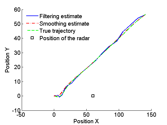
figure('name', 'SMC: Filtering and smoothing estimates')
x_f_mean = summ_smc.x.f.mean;
x_s_mean = summ_smc.x.s.mean;
plot(x_f_mean(1, :), x_f_mean(2, :))
hold on
plot(x_s_mean(1, :), x_s_mean(2, :), '-.r')
plot(x_pos_true(1,:), x_pos_true(2,:), '--g')
plot(x_pos(1), x_pos(2), 'sk')
legend('Filtering estimate', 'Smoothing estimate', 'True trajectory',...
    'Position of the radar', 'location', 'Northwest')
legend boxoff
xlabel('Position X')
ylabel('Position Y')
box off

Plot particles

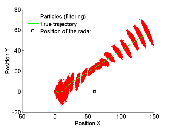
figure('name', 'SMC: Particles (filtering)')
plot(out_smc.x.f.values(1,:), out_smc.x.f.values(2,:), 'ro', ...
    'markersize', 2, 'markerfacecolor', 'r')
hold on
plot(x_pos_true(1,:), x_pos_true(2,:), '--g')
plot(x_pos(1), x_pos(2), 'sk')
legend('Particles (filtering)', 'True trajectory', 'Position of the radar', 'location', 'Northwest')
legend boxoff
xlabel('Position X')
ylabel('Position Y')
box off

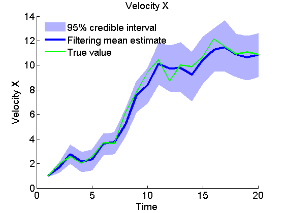
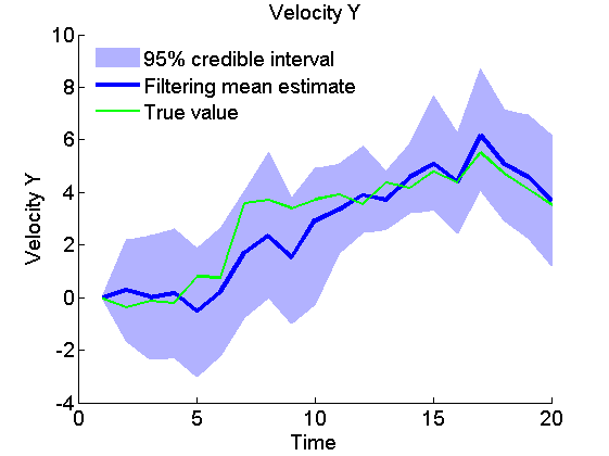
Plot Filtering estimates

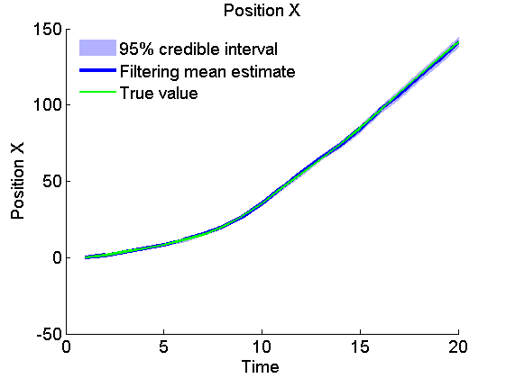
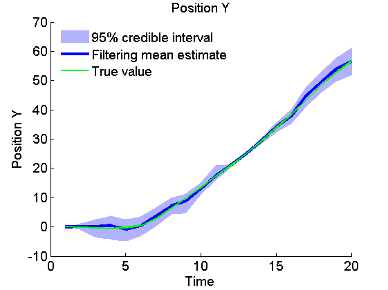
x_f_quant = summ_smc.x.f.quant;
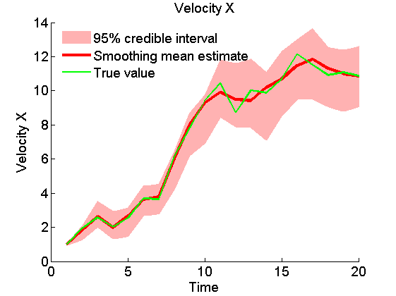
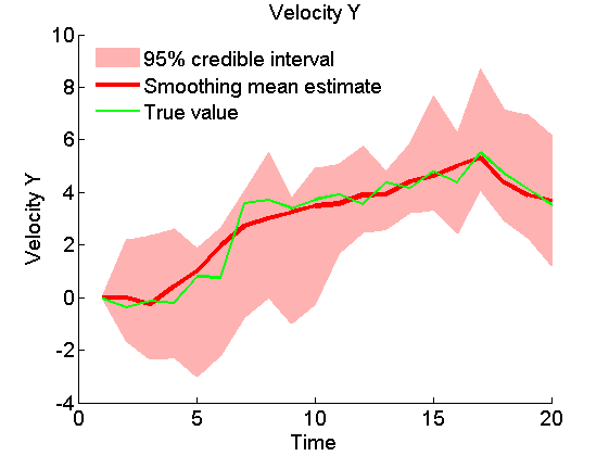
title_fig = {'Position X', 'Position Y', 'Velocity X', 'Velocity Y'};
for k=1:4
    figure('name', 'SMC: Filtering estimates')
    title(title_fig{k})
    hold on
    h = fill([1:t_max, t_max:-1:1], [x_f_quant{1}(k,:), fliplr(x_f_quant{2}(k,:))], 0);
    set(h, 'edgecolor', 'none', 'facecolor', light_blue)
    plot(x_f_mean(k, :), 'linewidth', 3)
    plot(data.x_true(k,:), 'g')
    xlabel('Time')
    ylabel(title_fig{k})
    legend({'95% credible interval', 'Filtering mean estimate', 'True value'},...
        'location', 'Northwest')
    legend boxoff
    box off
end

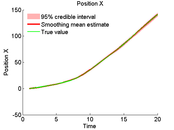
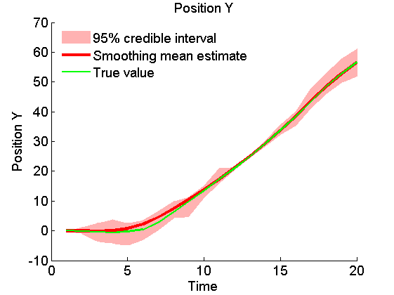
Plot Smoothing estimates

x_s_quant = summ_smc.x.s.quant;
for k=1:4
    figure('name', 'SMC: Smoothing estimates')
    title(title_fig{k})
    hold on
    h = fill([1:t_max, t_max:-1:1], [x_f_quant{1}(k,:), fliplr(x_f_quant{2}(k,:))], 0);
    set(h, 'edgecolor', 'none', 'facecolor', light_red)
    plot(x_s_mean(k, :), 'r', 'linewidth', 3)
    plot(data.x_true(k,:), 'g')
    xlabel('Time')
    ylabel(title_fig{k})
    legend({'95% credible interval', 'Smoothing mean estimate', 'True value'},...
        'location', 'Northwest')
    legend boxoff
    box off
end

Clear model

biips_clear()

Published with MATLAB® R2014a